
The g Factor: The Science of Mental Ability
Arthur R. Jensen, 1998.
Chapter 4 : Models and Characteristics of g
STATISTICAL SAMPLING ERROR
The size of g, that is, the proportion of the total variance that g accounts for in any given battery of tests, depends to some extent on the statistical characteristics of the group tested (as compared with a large random sample of the general population). Most factor analytic studies of tests reported in the literature are not based on representative samples of the general population. Rather, subject samples are usually drawn from some segment of the population (often college students or military trainees) that does not display either the mean level of mental ability or the range of mental ability that exists in the total population. Because g is by far the most important ability factor in determining the aggregation of people into such statistically distinguishable groups, the study groups will be more homogeneous in g than in any other ability factors. Hence when the g factor is extracted, it is actually smaller than it would be if extracted from data for the general population. Relative to other factors, g is typically underestimated in most studies. This is especially so in samples drawn from the students at the most selective colleges and universities, where admission is based on such highly g-loaded criteria as superior grades in high school and high scores on scholastic aptitude tests.
Many factor analytic studies have been based on recruits in the military, which is a truncated sample of the population, with the lower 10 percent (i.e., IQs below 80) excluded by congressional mandate. Also, the various branches of the armed services differ in their selection criteria based in part on mental test scores (rejecting the lowest-scoring 10 to 30 percent), with consequently different range restrictions of g.
The samples most representative of the population are the large samples used to standardize most modern IQ tests and the studies of elementary schoolchildren randomly sampled from urban, suburban, and rural schools. Because the dropout rate increases with grade level and is inversely related to IQ, high school students are a somewhat more g-restricted sample of the general population.
A theoretically interesting phenomenon is that g accounts for less of the variance in a battery of tests for the upper half of the population distribution of IQ than for the lower half, even though the upper and lower halves do not differ in the range of test scores or in their variance. [11] The basis of g is that the correlations among a variety of tests are all positive. Since the correlations are smaller, on average, in the upper half than in the lower half of the IQ distribution, it implies that abilities are more highly differentiated in the upper half of the ability distribution. That is, relatively more of the total variance consists of group factors and the tests’ specificity, and relatively less consists of g for the upper half of the IQ distribution than for the lower half. (For a detailed discussion of this phenomenon, see Appendix A.)
Specificity (s) is the least consistent characteristic of tests across different factor analyses, because the amount of specific variance in a test is a function of the number and the variety of the other tests in the factor analysis. Holding constant the number of tests, the specificity of each test increases as the variety of the tests in the battery increases. As variety decreases, or the more that the tests in a battery are made to resemble one another, the variance that would otherwise constitute specificity becomes common factor variance and forms group factors. If the variety of tests in a battery is held constant, specificity decreases as the number of tests in the battery is increased. As similar tests are added, they contribute more to the common factor variance (g + group factors), leaving less residual variance (which includes specificity).
As more and more different tests are included in a battery, each newly added test has a greater chance of sharing the common factor variance, thereby losing some of its specificity. For example, if a battery of tests includes the ubiquitous g and three group factors but includes only one test of short-term memory (e.g., digit span), that test’s variance components will consist only of g plus s plus error. If at least two more tests of short-term memory (say, word span and repetition of sentences) are then added to this battery, the three short-term memory tests will form a group factor. Most of what was the digit span test’s specific variance, when it stood alone in the battery, is now aggregated into a group factor (composed of digit span, word span, and repetition of sentences), leaving little residual specificity in each of these related tests.
Theoretically, the only condition that limits the transformation of specific variance into common factor variance when new tests are added or existing tests are made more alike is the reliability of the individual test scores. When the correlation between any two or more tests is as high as their reliability coefficients will allow (the square root of the product of the tests’ reliability coefficients is the mathematical upper bound), they no longer qualify as separate tests and cannot legitimately be used in the same factor analysis to create another group factor. A group factor created in this manner is considered spurious. But there are also some nonspurious group factors that are so small and inconsistently replicable across different test batteries or different population samples that they are trivial, theoretically and practically.
PSYCHOMETRIC SAMPLING ERROR
How invariant is the g extracted from different collections of tests when the method of factor analysis and the subject sample remain constant? There is no method of factor analysis that can yield exactly the same g when different tests are included in the battery. As John B. Carroll (1993a, p. 596) aptly put it, the g factor is “colored” or “flavored” by its ingredients, which are the tests or primary factors whose variance is dominated by g. The g is always influenced, more or less, by both the nature and the variety of the tests from which it is extracted. If the g extracted from different batteries of tests was not substantially consistent, however, g would have little theoretical or practical importance as a scientific construct. But the fact is that g remains quite invariant across many different collections of tests.
It should be recognized, of course, that in factor analysis, as in every form of measurement in science, either direct or indirect (e.g., through logical inference), there are certain procedural rules that must be followed if valid measures are to be obtained. The accuracy of quantitative analysis in chemistry, for example, depends on using reagents of standardized purity. Similarly, in factor analysis, the extraction of g depends on certain requirements for proper psychometric sampling.
The number of tests is the first consideration. The extraction of g as a second-order factor in a hierarchical analysis requires a minimum of nine tests from which at least three primary factors can be obtained.
That three or more primary factors are called for implies the second requirement: a variety of tests (with respect to their information content, skills, and task demands on a variety of mental operations) is needed to form at least three or more distinct primary factors. In other words, the particular collection of tests used to estimate g should come as close as possible, with some limited number of tests, to being a representative sample of all types of mental tests, and the various kinds of tests should be represented as equally as possible. If a collection of tests appears to be quite limited in variety, or is markedly unbalanced in the varieties it contains, the extracted g is probably contaminated by non-g variance and is therefore a poor representation of true g.
If we factor-analyzed a battery consisting, say, of ten kinds of numerical tests, two tests of verbal reasoning, and one test of spatial reasoning, for example, we would obtain a quite distorted g. The general factor (or nominal g) of this battery would actually consist of g plus some sizable admixture of a numerical ability factor. Therefore, this nominal g would differ considerably from another nominal g obtained from a battery consisting of, say, ten verbal tests, two spatial reasoning tests, and one numerical test. The nominal g of this second battery would really consist of g plus a large admixture of verbal ability.
The problem of contamination is especially significant when one extracts g as the first factor (PF1) in a principal factor analysis. The largest PF1 loadings that emerge are all on tests of the same type, so a marked imbalance in the types of tests entering into the analysis will tend to distort the PF1 as a representation of g. If there are enough tests to permit a proper hierarchical analysis, however, an imbalance in the variety of tests is overcome to a large extent by the aggregation of the overrepresented tests into a single group factor. This factor then carries a weight that is more equivalent to the other group factors (which are based on fewer tests), and it is from the correlations among the group factors that the higher-order g is derived. This is one of the main advantages of a hierarchical analysis.
Ability Variation between Persons and within Persons. It is sometimes claimed that any given person shows such large differences in various abilities that it makes no sense to talk about general ability, or to attempt to represent it by a single score, or to rank persons on it. One student does very well in math, yet has difficulty with English composition; another is just the opposite; a third displays a marked talent for music but is mediocre in English and math. Is this a valid argument against g? It turns out that it is not valid, for if it were true, it would not be possible to demonstrate repeatedly the existence of all-positive correlations among scores on diverse tests abilities, or to obtain a g factor in a hierarchical factor analysis. At most, there would only be uncorrelated group factors, and one could orthogonally rotate the principal factor axes to virtually perfect simple structure.
A necessary implication of the claim that the levels of different abilities possessed by an individual are so variable as to contradict the idea of general ability is that the differences between various abilities within persons would, on average, be larger than the differences between persons in the overall average of these various abilities. This proposition can be (and has been) definitively tested by means of the statistical method known as the analysis of variance. The method is most easily explained with the following type of “Tests x Persons” matrix.
It shows ten hypothetical tests of any diverse mental abilities (A, B , . . . J) administered to a large number, N, of persons. The test scores have all been standardized (i.e., converted to z scores) so that every test has a mean z = 0 and standard deviation = 1. Therefore, the mean score on every test (i.e., Mean T in the bottom row) is the same (i.e., Mean = 0). Hence there can be only three sources of variance in this whole matrix: (1) the differences between persons’ (P) mean scores on the ten tests (Mean P [z1, z2, z3, etc.] in last column), and (2) the differences between test scores within each person (e.g., the zA1, zB1, zC1, etc., are the z scores on Tests A, B, C, etc., for Person 1). Now, if the average variance within persons proves to be as large as or larger than the variance between persons, one could say there is no overall general level of ability, or g, in which people differ. That is, differences in the level of various abilities within a person are as large or larger, on average, than differences between persons in the overall average level of these various abilities. In fact, just the opposite is empirically true: Differences in the average level of abilities between persons are very significantly greater than differences in various abilities within persons.
It should be remembered that g and all other factors derived from factor analysis depend essentially on variance between persons. Traits in which there is very little or no variance do not show up in a factor analysis. A small range of variation in the measurements subjected to factor analysis may result in fewer and smaller factors. A factor analysis performed on the fairly similar body measurements of all the Miss Universe contestants (or of heavyweight boxers), for example, would yield fewer and much smaller factors than the same analysis performed on persons randomly selected from the general population.
Chapter 5 : Challenges to g
VERBAL ARGUMENTS
THE SPECIFICITY DOCTRINE
If the only source of individual differences is past learning, it is hard to explain why individual differences in a variety of tasks that are so novel to all of the subjects as to scarcely reflect the transfer of training from prior learned skills or problem-solving strategies are still highly correlated. Transfer from prior learning is quite task-specific. It is well known, for example, that memory span for digits (i.e., repeating a string of n random digits after hearing them spoken at a rate of one digit per second) has a moderate correlation with IQ. It also has a high correlation with memory span for random consonant letters presented in the same way. The average memory span in the adult population is about seven digits, or seven consonant letters. (The inclusion of vowels permits the grouping of letters into pronounceable syllables, which lengthens the memory span.) Experiments have been performed in which persons are given prolonged daily practice in digit span memory over a period of several months. Digit span memory increases remarkably with practice; some persons eventually become able to repeat even 70 to 100 digits without error after a single presentation. [3] But this developed skill shows no transfer effect on IQ, provided the IQ test does not include digit span. But what is even more surprising is that there is no transfer to letter span memory. Persons who could repeat a string of seven letters before engaging in practice that raised their digit span from seven to 70 or more digits still have a letter span of about seven letters. Obviously, practicing one kind of task does not affect any general memory capacity, much less g.
What would happen to the g loadings of a battery of cognitive tasks if they were factor analyzed both before and after subjects had been given prolonged practice that markedly improved their performance on all tasks of the same kind? I know of only one study like this, involving a battery of cognitive and perceptual-motor skill tasks. [4] Measures of task performance taken at intervals during the course of practice showed that the tasks gradually lost much of their g loading as practice continued, and the rank order of the tasks’ pre- and post-practice g loadings became quite different. Most striking was that each task’s specificity markedly increased. Thus it appears that what can be trained up is not the g factor common to all tasks, but rather each task’s specificity, which reflects individual differences in the specific behavior that is peculiar to each task. By definition a given task’s specificity lacks the power to predict performance significantly on any other tasks except those that are very close to the given task on the transfer gradient.
The meager success of skills training designed for persons scoring below average on typical g-loaded tests illustrates the limited gain in job competence that can be obtained when specific skills are trained up, leaving g unaffected. In the early 1980s, for example, the Army Basic Skills Education Program was spending some $40 million per year to train up basic skills for the 10 percent of enlisted men who scored below the ninth-grade level on tests of reading and math, with up to 240 hours of instruction lasting up to three months. The program was motivated by the finding that recruits who score well on tests of these skills learn and perform better than low scorers in many army jobs of a technical nature. An investigation of the program’s outcomes by the U.S. General Accounting Office (G.A.O.), however, discovered very low success rates. […]
… Is there any principle of learning or transfer that would explain or predict the high correlations between such dissimilar tasks as verbal analogies, number series, and block designs? Could it explain or predict the correlation between pitch discrimination ability and visual perceptual speed, or the fact that they both are correlated with each of the three tests mentioned above?
“Intelligence” as Learned Behavior. If the only source of individual differences is past learning, it is hard to explain why individual differences in a variety of tasks that are so novel to all of the subjects as to scarcely reflect the transfer of training from prior learned skills or problem-solving strategies are still highly correlated. Transfer from prior learning is quite task-specific. It is well known, for example, that memory span for digits (i.e., repeating a string of n random digits after hearing them spoken at a rate of one digit per second) has a moderate correlation with IQ. It also has a high correlation with memory span for random consonant letters presented in the same way. The average memory span in the adult population is about seven digits, or seven consonant letters. (The inclusion of vowels permits the grouping of letters into pronounceable syllables, which lengthens the memory span.) Experiments have been performed in which persons are given prolonged daily practice in digit span memory over a period of several months. Digit span memory increases remarkably with practice; some persons eventually become able to repeat even 70 to 100 digits without error after a single presentation. [3] But this developed skill shows no transfer effect on IQ, provided the IQ test does not include digit span. But what is even more surprising is that there is no transfer to letter span memory. Persons who could repeat a string of seven letters before engaging in practice that raised their digit span from seven to 70 or more digits still have a letter span of about seven letters. Obviously, practicing one kind of task does not affect any general memory capacity, much less g.
SAMPLING THEORIES OF THORNDIKE AND THOMSON
[…] More complex tests are highly correlated and have larger g loadings than less complex tests. This is what one would predict from the sampling theory: a complex test involves more neural elements and would therefore have a greater probability of involving more elements that are common to other tests.
But there are other facts the overlapping elements theory cannot adequately explain. One such question is why a small number of certain kinds of nonverbal tests with minimal informational content, such as the Raven matrices, tend to have the highest g loadings, and why they correlate so highly with content-loaded tests such as vocabulary, which surely would seem to tap a largely different pool of neural elements. Another puzzle in terms of sampling theory is that tests such as forward and backward digit span memory, which must tap many common elements, are not as highly correlated as are, for instance, vocabulary and block designs, which would seem to have few elements in common. Of course, one could argue trivially in a circular fashion that a higher correlation means more elements in common, even though the theory can’t tell us why seemingly very different tests have many elements in common and seemingly similar tests have relatively few.
Even harder to explain in terms of the sampling theory is the finding that individual differences on a visual scan task (i.e., speed of scanning a set of digits for the presence or absence of a “target” digit), which makes virtually no demand on memory, and a memory scan test (i.e., speed of scanning a set of digits held in memory for the presence or absence of a “target” digit) are perfectly correlated, even though they certainly involve different neural processes. [21] And how would sampling theory explain the finding that choice reaction time is more highly correlated with scores on a nonspeeded vocabulary test than with scores on a test of clerical checking speed? Another apparent stumbling block for sampling theory is the correlation between neural conduction velocity (NCV) in a low-level brain tract (from retina to primary visual cortex) and scores on a complex nonverbal reasoning test (Raven), even though the higher brain centers that are engaged in the complex reasoning ability demanded by the Raven do not involve the visual tract.
Perhaps the most problematic test of overlapping neural elements posited by the sampling theory would be to find two (or more) abilities, say, A and B, that are highly correlated in the general population, and then find some individuals in whom ability A is severely impaired without there being any impairment of ability B. For example, looking back at Figure 5.2, which illustrates sampling theory, we see a large area of overlap between the elements in Test A and the elements in Test B. But if many of the elements in A are eliminated, some of its elements that are shared with the correlated Test B will also be eliminated, and so performance on Test B (and also on Test C in this diagram) will be diminished accordingly. Yet it has been noted that there are cases of extreme impairment in a particular ability due to brain damage, or sensory deprivation due to blindness or deafness, or a failure in development of a certain ability due to certain chromosomal anomalies, without any sign of a corresponding deficit in other highly correlated abilities. [22] On this point, behavioral geneticists Willerman and Bailey comment: “Correlations between phenotypically different mental tests may arise, not because of any causal connection among the mental elements required for correct solutions or because of the physical sharing of neural tissue, but because each test in part requires the same ‘qualities’ of brain for successful performance. For example, the efficiency of neural conduction or the extent of neuronal arborization may be correlated in different parts of the brain because of a similar epigenetic matrix, not because of concurrent functional overlap.” [22] A simple analogy to this would be two independent electric motors (analogous to specific brain functions) that perform different functions both running off the same battery (analogous to g). As the battery runs down, both motors slow down at the same rate in performing their functions, which are thus perfectly correlated although the motors themselves have no parts in common. But a malfunction of one machine would have no effect on the other machine, although a sampling theory would have predicted impaired performance for both machines.
GARDNER’S SEVEN “FRAMES OF MIND” AND MENTAL MODULES
In fact, it is hard to justify calling all of the abilities in Gardner’s system by the same term — “intelligences.” If Gardner claims that the various abilities he refers to as “intelligences” are unrelated to one another (which has not been empirically demonstrated), what does it add to our knowledge to label them all “intelligences”? … Bobby Fisher, then, could be claimed as one of the world’s greatest athletes, and many sedentary chess players might be made to feel good by being called athletes. But who would believe it? The skill involved in chess isn’t the kind of thing that most people think of as athletic ability, nor would it have any communality if it were entered into a factor analysis of typical athletic skills. […]
Modular Abilities. Gardner invokes recent neurological research on brain modules in support of his theory. [35] But there is nothing at all in this research that conflicts in the least with the findings of factor analysis. It has long been certain that the factor structure of abilities is not unitary, because factor analysis applied to the correlations among any large and diverse battery of ability tests reveals that a number of factors (although fewer than the number of different tests) must be extracted to account for most of the variance in all of the tests. The g factor, which is needed theoretically to account for the positive correlations between all tests, is necessarily unitary only within the domain of factor analysis. But the brain mechanisms or processes responsible for the fact that individual differences in a variety of abilities are positively correlated, giving rise to g, need not be unitary. […]
Some of the highly correlated abilities identified as factors probably represent what are referred to as modules. But here is the crux of the main confusion, which results when one fails to realize that in discussing the modularity of mental abilities we make a transition from talking about individual differences and factors to talking about the localized brain processes connected with various kinds of abilities. Some modules may be reflected in the primary factors; but there are other modules that do not show up as factors, such as the ability to acquire language, quick recognition memory for human faces, and three-dimensional space perception, because individual differences among normal persons are too slight for these virtually universal abilities to emerge as factors, or sources of variance. This makes them no less real or important. Modules are distinct, innate brain structures that have developed in the course of human evolution. They are especially characterized by the various ways that information or knowledge is represented by the neural activity of the brain. The main modules thus are linguistic (verbal/auditory/lexical/semantic), visuospatial, object recognition, numerical-mathematical, musical, and kinesthetic.
Although modules generally exist in all normal persons, they are most strikingly highlighted in two classes of persons, (a) those with highly localized brain lesions. Or pathology, and (b) idiots savants. Savants evince striking discrepancies between amazing proficiency in a particular narrow ability and nearly all other abilities, often showing an overall low level of general ability. Thus we see some savants who are even too mentally retarded to take care of themselves, yet who can perform feats of mental calculation, or play the piano by ear, or memorize pages of a telephone directory, or draw objects from memory with photographic accuracy. The modularity of these abilities is evinced by the fact that rarely, if ever, is more than one of them seen in a given savant.
In contrast, there are persons whose tested general level of ability is within the normal range, yet who, because of a localized brain lesion, show a severe deficiency in some particular ability, such as face recognition, receptive or expressive language dysfunctions (aphasia), or inability to form long-term memories of events. Again, modularity is evidenced by the fact that these functional deficiencies are quite isolated from the person’s total repertoire of abilities. Even in persons with a normally intact brain, a module’s efficiency can be narrowly enhanced through extensive experience and practice in the particular domain served by the module.
Such observations have led some researchers to the mistaken notion that they contradict the discovery of factor analysis that, in the general population, individual differences in mental abilities are all positively and hierarchically correlated, making for a number of distinct factors and a higher-order general factor, or g. The presence of a general factor indicates that the workings of the various modules, though distinct in their functions, are all affected to some degree by some brain characteristic(s), such as chemical neurotransmitters, neural conduction velocity, amount of dendritic branching, and degree of myelination of axons, in which there are individual differences. Hence individual differences in the specialized mental activities associated with different modules are correlated.
A simple analogy might help to explain the theoretical compatibility between the positive correlations among all mental abilities and the existence of modularity in mental abilities. Imagine a dozen factories (“persons”), each of which manufactures the same five different gadgets (“modular abilities”). Each gadget is produced by a different machine (“module”). The five machines are all connected to each other by a gear chain that is powered by one motor. But each of the five factories uses a different motor to drive the gear chain, and each factory’s motor runs at a constant speed different from the speed of the motors in any other factory. This will cause the factories to differ in their rates of output of the five gadgets (“scores on five different tests”). The factories will be said to differ in overall efficiency or capacity, because the rates of output of the five gadgets are positively correlated. If the correlations between output rates of the gadgets produced by all five factories were factor analyzed, they would yield a large general factor. Gadgets’ output rates may not be perfectly correlated, however, because the sales demand for each gadget differs across factories, and the machines that produce the gadgets with the larger sales are better serviced, better oiled, and kept in consistently better operating condition than the machines that make low-demand gadgets. Therefore, even though the five machines are all driven by the same motor, they differ somewhat in their efficiency and consistency of operation, making for less than a perfect correlation between the rates of output. Now imagine that in one factory the main drive shaft of one of the machines breaks, and it cannot produce its gadget at all (analogous to localized brain damage affecting a single module, but not g). In another factory, four of the machines break down and fail to produce gadgets, but one machine is very well maintained because it continues to run and puts out gadgets at a rate commensurate with the speed of the motor that powers the gear chain that runs the machine (analogous to an idiot savant).
Chapter 6 : Biological Correlates of g
SPECIFIC BIOLOGICAL CORRELATES OF IQ AND g
Body Size (Extrinsic). It is now well established that both height and weight are correlated with IQ. When age is controlled, the correlations in different studies range mostly between +.10 and +.30, and average about +.20. Studies based on siblings find no significant within-family correlation, and gifted children (who are taller than their age mates in the general population) are not taller than their nongifted siblings.
Because both height and IQ are highly heritable, the between-families correlation of stature and IQ probably represents a simple genetic correlation resulting from cross-assortative mating for the two traits. Both height and “intelligence” are highly valued in Western culture and it is known that there is substantial assortative mating for each trait.
There is also evidence of cross-assortative mating for height and IQ; there is some trade-off between them in mate selection. When short and tall women are matched on IQ, educational level, and social class of origin, for example, it is found that the taller women tend to marry men of higher intelligence (reasonably inferred from their higher educational and occupational status) than do shorter women. Leg length relative to overall height is regarded an important factor in judging feminine beauty in Western culture, and it is interesting that the height x IQ correlation is largely attributable to the leg-length component of height. Sitting height is much less correlated with IQ. If there is any intrinsic component of the height x IQ correlation, it is too small to be detected at a significant level even in quite large samples. The two largest studies [8] totaling some 16,000 sibling pairs, did not find significant within-family correlations of IQ with either height or weight (controlling for age) in males or females or in blacks or whites.
Head Size and Brain Size (Intrinsic). There is a great deal of evidence that external measurements of head size are significantly correlated with IQ and other highly g-loaded tests, although the correlation is quite small, in most studies ranging between +.10 and +.25, with a mean r ≈ +.15. The only study using g factor scores showed a correlation of +.30 with a composite measure of head size based on head length, width, and circumference, in a sample of 286 adolescents. [9] Therefore, it appears that head size is mainly correlated with the g component of psychometric scores. The method of correlated vectors applied to the same sample of 286 adolescents showed a highly significant rs = +.64 between the g vector of seventeen diverse tests and the vector of the tests’ correlations with head size. The head-size vector had nonsignificant correlations with the vectors of the spatial, verbal, and memory factors of +.27, .00, and +.05, respectively.
In these studies, of course, head size is used as merely a crude proxy for brain size. The external measurement of head size is in fact a considerably attenuated proxy for brain size.
The correlation between the best measures of external head size and actual brain size as directly measured in autopsy is far from perfect, being around +.50 to +.60 in adults and slightly higher in children. There are specially devised formulas by which one can estimate internal cranial capacity (in cubic centimeters) from external head measurements with a fair degree of accuracy. These formulas have been used along with various statistical corrections for age, body size (height, weight, total surface area), and sex to estimate the correlation between IQ and brain size from data on external head size. The typical result is a correlation of about .30.
These indirect methods, however, are no longer necessary, since the technology of magnetic resonance imaging (MRI) now makes it possible to obtain a three-dimensional picture of the brain of a living person. A highly accurate measure of total brain volume (or the volume of any particular structure in the brain) can be obtained from the MRI pictures. Such quantitative data are now usually extracted from the MRI pictures by computer.
To date there are eight MRI studies [10] of the correlation between total brain volume and IQ in healthy children and young adults. In every study the correlations are significant and close to +.40 after removing variance due to differences in body size. (The correlation between body size and brain size in adult humans is between +.20 and +.25.) Large parts of the brain do not subserve cognitive processes, but govern sensory and motor functions, emotions, and autonomic regulation of physiological activity. Controlling body size removes to some extent the sensorimotor aspects of brain size from the correlation of overall brain size with IQ. But controlling body size in the brain X IQ correlation is somewhat problematic, because there may be some truly functional relationship between brain size and body size that includes the brain’s cognitive functions. Therefore, controlling body size in the IQ X brain size correlation may be too conservative; it could result in overcorrecting the correlation. Moreover, the height and weight of the head constitute an appreciable proportion of the total body height and weight, so that controlling total body size could also contribute to overcorrection by removing some part of the variance in head and brain size along with variance in general body size. Two of the MRI studies used a battery of diverse cognitive tests, which permitted the use of correlated vectors to determine the relationship between the column vector of the varioustests’ g factor loadings and the column vector of the tests’ correlations with total brain volume. In one study, [10f] based on twenty cognitive tests given to forty adult males sibling pairs, these vectors were correlated +.65. In the other study, [10g] based on eleven diverse cognitive tests, the vector of the tests’ g loadings were correlated +.51 with the vector of the tests’ correlations with total brain volume and +.66 with the vector of the tests’ correlations with the volume of the brain’s cortical gray matter. In these studies, all of the variables entering into the analyses were the averages of sibling pairs, which has the effect of increasing the reliability of the measurements. Therefore, these analyses are between-families. A problematic aspect of both studies is that there were no significant within-family correlations between test scores and brain volumes, which implies that there is no intrinsic relationship between brain size and g. To conclude that the within-family correlation in the population is zero, however, has a high risk of being a Type II error, given the unreliability of sibling difference scores (on which within-family correlations are based) and the small number of subjects used in these studies. Much larger studies based merely on external head size show significant within-family correlations with IQ. Clearly, further MRI studies are needed for a definitive answer on this critical issue.
Metabolically, the human brain is by far the most “expensive” organ in the whole body, and the body may have evolved to serve in part like a “power pack” for the brain, with a genetically larger brain being accommodated by a larger body. It has been determined experimentally, for example, that strains of rats that were selectively bred from a common stock exclusively to be either good or poor at maze learning were found to differ not only in brain size but also in body size. [11] Body size increased only about one-third as much as brain size as a result of the rats being selectively bred exclusively for good or poor maze-learning ability. There was, of course, no explicit selection for either brain size or body size, but only for maze-learning ability. Obviously, there is some intrinsic functional and genetic relationship between learning ability, brain size, and body size, at least in laboratory rats. Although it would be unwarranted to generalize this finding to humans, it does suggest the hypothesis that a similar relationship may exist in humans. It is known that body size has increased along with brain size in the course of human evolution. The observed correlations between brain size, body size, and mental ability in humans are consistent with these facts, but the nature and direction of the causal connections between these variables cannot be inferred without other kinds of evidence that is not yet available.
The IQ X head-size correlation is clearly intrinsic, as shown by significant correlations both between-families (r = +.20, p < .001) and within-families (r = +.11, p < .05) in a large sample of seven-year-old children, with head size measured only by circumference and IQ measured by the Wechsler Intelligence Scale for Children. [12] (Age, height, and weight were statistically controlled.) The same children at four years of age showed no significant correlation of head size with Stanford-Binet IQ, and in fact the WF correlation was even negative (-.04). This suggests that the correlation of IQ with head size (and, by inference, brain size) is a developmental phenomenon, increasing with age during childhood.
One of the unsolved mysteries regarding the relation of brain size to IQ is the seeming paradox that there is a considerable sex difference in brain size (the adult female brain being about 100 cm3 smaller than the male) without there being a corresponding sex difference in IQ. [13] It has been argued that some IQ tests have purposely eliminated items that discriminate between the sexes or have balanced-out sex differences in items or subtests. This is not true, however, for many tests such as Raven’s matrices, which is almost a pure measure of g, yet shows no consistent or significant sex difference. Also, the differing g loadings of the subscales of the Wechsler Intelligence Test are not correlated with the size of the sex difference on the various subtests. [14] The correlation between brain size and IQ is virtually the same for both sexes.
The explanation for the well-established mean sex difference in brain size is still somewhat uncertain, although one hypothesis has been empirically tested, with positive results. Properly controlling (by regression) the sex difference in body size diminishes, but by no means eliminates, the sex difference in brain size. Three plausible hypotheses have been proposed to explain the sex difference (of about 8 percent) in average brain size between the sexes despite there being no sex difference in g:
1. Possible sexual dimorphism in neural circuitry or in overall neural conduction velocity could cause the female brain to process information more efficiently.
2. The brain size difference could be due to the one ability factor, independent of g, that unequivocally shows a large sex difference, namely, spatial visualization ability, in which only 25 percent of females exceed the male median. Spatial ability could well depend upon a large number of neurons, and males may have more of these “spatial ability” neurons than females, thereby increasing the volume of the male brain.
3. Females have the same amount of functional neural tissue as males but there is a greater “packing density” of the neurons in the female brain. While the two previous hypotheses remain purely speculative at present, there is recent direct evidence for a sex difference in the “packing density” of neurons. [15] In the cortical regions most directly related to cognitive ability, the autopsied brains of adult women possessed, on average, about 11 percent more neurons per unit volume than were found in the brains of adult men. The males and females were virtually equated on Wechsler Full Scale IQ (112.3 and 110.6, respectively). The male brains were about 12.5 percent heavier than the female brains. Hence the greater neuronal packing density in the female brain nearly balances the larger size of the male brain. Of course, further studies based on histological, MRI, and PET techniques will be needed to establish the packing density hypothesis as the definitive explanation for the seeming paradox of the two sexes differing in brain size but not differing in IQ despite a correlation of about +.40 between these variables within each sex group.
Cerebral Glucose Metabolism. The brain’s main source of energy is glucose, a simple sugar. Its rate of uptake and subsequent metabolism by different regions of the brain can serve as an indicator of the degree of neural energy expended in various locations of the brain during various kinds of mental activity. This technique consists of injecting a radioactive isotope of glucose (F-18 deoxyglucose) into a person’s bloodstream, then having the person engage in some mental activity (such as taking an IQ test) for about half an hour, during which the radioactive glucose is metabolized by the brain. The isotope acts as a radioactive tracer of the brain’s neural activity.
Immediately following the uptake period in which the person was engaged in some standardized cognitive task, the gamma rays emitted by the isotope from the nerve cells in the cerebral cortex can be detected and recorded by means of a brain-scanning technique called positron emission tomography (or PET scan). The PET scan provides a picture, or map, of the specific cortical location and the amount of neural metabolism (of radioactive glucose) that occurred during an immediately preceding period of mental activity.
Richard J. Haier, a leading researcher in this field, has written a comprehensive review [26a] of the use of the PET scan for studying the physiological basis of individual differences in mental ability. The main findings can be summarized briefly. Normal adults have taken the Raven Advanced Progressive Matrices (RAPM) shortly after they were injected with radioactive glucose. The RAPM, a nonverbal test of reasoning ability, is highly g loaded and contains little, if any, other common factor variance. The amount of glucose metabolized during the thirty-five-minute testing period is significantly and inversely related to scores on the RAPM, with negative correlations between -.7 and -.8. In solving RAPM problems of a given level of difficulty, the higher-scoring subjects use less brain energy than the lower-scoring subjects, as indicated by the amount of glucose uptake. Therefore, it appears that g is related to the efficiency of the neural activity involved in information processing and problem solving. Negative correlations between RAPM scores and glucose utilization are found in every region of the cerebral cortex, but are highest in the temporal regions, both left and right.
The method of correlated vectors shows that g is specifically related to the total brain’s glucose metabolic rate (GMR) while engaged in a mental activity over a period of time. In one of Haier’s studies, [26b] the total brain’s GMR was measured immediately after subjects had taken each of the eleven subtests of the Wechsler Adult Intelligence Scale-Revised (WAIS-R), and the GMR was correlated with scores on each of the subtests. The vector of these correlations was correlated r = -.79 (rs = -.66, p < .05) with the corresponding vector of the subtests’ g loadings (based on the national standardization sample).
A phenomenon that might be called “the conservation of g” and has been only casually observed in earlier research, but has not yet been rigorously established by experimental studies, is at least consistent with the findings of a clever PET-scan study by Haier and co-workers. The “conservation of g” refers to the phenomenon that as people become more proficient in performing certain complex mental tasks through repeated practice on tasks of the same type, the tasks become automatized, less g demanding, and consequently less g loaded. Although there remain individual differences in proficiency on the tasks after extensive practice, individual differences in performance may reflect less g and more task-specific factors. Something like this was observed in a study [26b] in which subjects’ PET scans were obtained after their first experience with a video game (Tetris) that calls for rapid and complex information processing, visual spatial ability, strategy learning, and motor coordination. Initially, playing the Tetris game used a relatively large amount of glucose. Daily practice on the video game for 30 to 45 minutes over the course of 30 to 60 days, however, showed greatly increasing proficiency in playing the game, accompanied by a decreasing uptake of glucose and a marked decrease in the correlation of the total brain glucose metabolic rate with g. In other words, the specialized brain activity involved in more proficient Tetris performance consumed less energy. Significantly, the rate of change in glucose uptake over the course of practice is positively correlated with RAPM scores. The performance of high-g subjects improved more from practice and they also gained greater neural metabolic efficiency during Tetris performance than subjects who were lower in g, as indexed by both the RAPM test and the Wechsler Adult Intelligence Scale.
Developmental PET scan studies in individuals from early childhood to maturity show decreasing utilization of glucose in all areas of the brain as individuals mature. In other words, the brain’s glucose uptake curve is inversely related to the negatively accelerated curve of mental age, from early childhood to maturity. The increase in the brain’s metabolic efficiency seems to be related to the “neural pruning,” or normal spontaneous decrease in synaptic density. The spontaneous decrease is greatest during the first several years of life. “Neural pruning” apparently results in greater efficiency of the brain’s capacity for information processing. Paradoxical as it may seem, an insufficient loss of neurons during early maturation is associated with some types of mental retardation.
Brain Nerve Conduction Velocity. Reed and Jensen (1992) measured NCV in the primary visual tract between the retina of the eye and the visual cortex in 147 college males and found a significant correlation of +.26 (p = .002) between NCV and Raven IQ. (The correlation is +.37 after correction for restriction of range of IQ in this sample of college students.) When the sample is divided into quintiles (five equal-sized groups) on the basis of the average velocity of the P100 visual evoked potential (V:P100), the average IQ in each quintile increases as a function of the V:P100 as shown in Figure 6.3.

A theoretically important aspect of this finding is that the NCV (i.e., V:P100) is measured in a brain tract that is not a part of the higher brain centers involved in the complex problem solving required by the Raven test, and the P100 visual evoked potential occurs, on average, about 100 milliseconds after the visual stimulus, which is less than the time needed for conscious awareness of the stimulus. This means that although the cortical NCV involved in Raven performance may be correlated with the NCV in the subcortical visual tract, the same neural elements are not involved. This contradicts Thomson’s sampling theory of g, which states that tests are correlated to the extent that they utilize the same neural elements. But here we have a correlation between the P100 visual evoked potential and scores on the Raven matrices that cannot be explained in terms of their overlapping neural elements. In the same subject sample, Reed and Jensen found that although NCV and choice reaction time (CRT) are both significantly correlated with IQ, they are not significantly correlated with each other. [33] This suggests two largely independent processes contributing to g, one linked to NCV and one linked to CRT. As this puzzling finding is based on a single study, albeit with a large sample, it needs to be replicated before much theoretical importance can be attached to it. There is other evidence that makes the relationship of NCV to g worth pursuing. For one thing, the pH level (hydrogen ion concentration) of the fluid surrounding a nerve cell is found experimentally to affect the excitability of the nerve, an increased pH level (i.e., greater alkalinity) producing a lower threshold of excitability. [34a] Also, a study of 42 boys, aged 6 to 13 years, found a correlation of .523 (p < .001) between a measure of intracellular brain pH and the WISC-III Full Scale IQ. [34b] Moreover, the method of correlated vectors shows that the vector of the 12 WISC subtests’ correlations with pH are significantly correlated with the vector of the subtests’ g loadings (r = +.63, rs = +.53, p < .05). This relationship of brain pH to g certainly merits further study.
Chapter 7 : The Heritability of g
IS g ONE AND THE SAME FACTOR BETWEEN FAMILIES AND WITHIN FAMILIES?
As we shall see, the main factor in the heritability of IQ and other mental tests is g. Also, as we shall see, genetic analysis and the calculation of heritability depend on a comparison of the trait variance between families (BF) and the variance within families (WF). (The separation of the total or population variance and correlation into BF and WF components was introduced in Chapter 6, pp. 141-42.) Therefore, before discussing the heritability of g, we must ask whether the g factor that emerges from a factor analysis of BF correlations is the very same g that emerges from a factor analysis of WF correlations. Recall that BF is the mean of all the full siblings (reared together) in each family in the population; WF is the differences among full siblings (reared together). In other words, some proportion of the total population variance (VP) in a trait measured on individuals is variance between families (VBF) and some proportion is variance within families (VWF). Thus theoretically VP = VBF + VWF. Similarly, the population correlation between any two variables reliably measured on individuals can be apportioned to BF and WF. The method for doing this requires measuring the variables of interest in sets of full siblings who were reared together.
Why might one expect the correlations between different mental tests, say X and Y, to be any different BF than WF? If the genetic or environmental influences that cause families to differ from one another on X or Y (or both) are of a different nature than the influences that cause differences on X or Y among siblings reared together in the same family, it would be surprising if the BF correlation of X and Y were the same as the WF correlation. And if there were a large number of diverse tests, the probability would be nil that all their intercorrelations would have the same factor structure in both BF and WF if the tests did not reflect the same causal variables acting to the same degree in both cases.
BF differences can be genetic or environmental, or both. A typical source of BF variance is social class or socioeconomic status (SES). Families differ in SES, but siblings reared in the same family do not differ in SES; therefore SES is not a source of WF variance. The same is true of differences associated with race, cultural identification, ethnic cuisines, and other such variables. They differ between families (BF) but seldom differ between full siblings reared together in the same household.
Now consider two sets of tests: A and B, X and Y. If the scores on Tests A and B are both strongly influenced by SES and other variables on which families differ and on which siblings in the same family do not differ, and if scores on Test X and Test Y are very little influenced by these BF variables, we should expect two things: (1) the BF correlation of A and B (rAB) would be larger than the BF correlation of X and Y (rXY), and (2) the BF correlation of A and B (rAB) would be unrelated to the BF correlation of X and Y (rXY). The greater size of the correlation rAB reflects similarity in the greater effect of SES (or other BF variables) on the scores of these two tests. This could be shown further by the fact that the BF correlation is much larger than the WF correlation for tests A and B. The size of the correlation rXY, on the other hand, reflects something other than SES (or other variables) on which families differ. So if the BF rXY and the WF rXY are virtually equal (after correction for attenuation [2]) and if this is also true of the BF and WF correlations for many diverse tests, it suggests that the same causal factors are involved in both the BF and WF correlations for these tests (unlike Tests A and B).
We can examine the hypothesis that the genetic and environmental influences that produce BF differences in tests’ g loadings are the same as the genetic and environmental influences that produce WF differences in the tests’ g loadings. If we find that this hypothesis cannot be rejected, we can rule out the supposed direct BF environmental influences on g, such as SES, racial-cultural differences, and the like. The observed mean differences between different SES, racial, and cultural groups on highly g-loaded tests then must be attributed to the same influences that cause differences among the siblings within the same families. As will be explicated later, these sibling differences result from both genetic and environmental (better called nongenetic) effects.
Two large-scale studies have tested this hypothesis. In each study, a g factor was extracted from the BF correlations among a number of highly diverse tests and also from the WF correlations among the same tests. [3] These two factors are referred to as gBF and gWF.
The first study [4] was based on pairs of siblings (nearest in age, in grades 2 to 6) from 1,495 white and 901 black families. They were all given seven highly diverse age-standardized tests (Memory, Figure Copying, Pictorial IQ, Nonverbal IQ, Verbal IQ, Vocabulary, and Reading Comprehension). Both BF and WF correlations among the tests were obtained separately for whites and blacks, and a g factor (first principal component) was extracted from each of the four correlation matrices. The degree of similarity between factors is properly assessed by the coefficient of congruence, rc. [5] Two factors with values of rc larger than .90 are generally interpreted as “highly similar”; values above .95 as having “virtual identity.” The values of rc are shown in Table 7.1. They are all very high and probably not significantly different from one another. The high congruence of the gBF and gWF factors in each racial group indicates that g is clearly an intrinsic factor (as defined in Chapter 6, p. 139). Also, both gBF and gWF are virtually the same across racial groups. In this California school population, little, if any, of the variance in the g factor in these tests is attributable to the effects of SES or cultural differences. Whatever SES and cultural differences may exist in this population do not alter the character of the general factor that all these diverse tests have in common.

The second study [6] is based on groups that probably have more distinct cultural differences than black and white schoolchildren in California, namely, teenage Americans of Japanese ancestry (AJA) and Americans of European ancestry (AEA), all living in Hawaii. Each group was composed of full siblings from a large number of families. They were all given a battery of fifteen highly diverse cognitive tests representing such first-order factors as verbal, spatial, perceptual speed and accuracy, and visual memory. In this study, the g factor was extracted as a second-order factor in a confirmatory hierarchical factor analysis. The same type of factor analysis was performed separately on the BF and WF correlations in each racial sample. The congruence coefficient between gBF and gWF was +.99 in both the AJA group and the AEA group, and the congruence across the AJA and AEA groups was +.99 for both gBF and gWF. These results are essentially the same as those in the previous study, even though the populations, tests, and methods of extracting the general factor all differed. Moreover, the four first-order group factors showed almost as high congruence between BF and WF and between AJA and AEA as did the second-order g factor. The authors of the second study, behavioral geneticists Craig Nagoshi and Ronald Johnson [6] concluded, “Nearly all of the indices used in the present analyses thus support a high degree of similarity in the factor structures of cognitive ability test scores calculated between versus within families. In other words, they suggest that the genetic and environmental factors underlying cognitive abilities are intrinsic in nature. These indices also suggest that these BF and WF structures are similar across the AEA and AJA ethnic groups, despite some earlier findings that may have led one to expect especially strong between-family effects for the AJA group” (p. 314).
EMPIRICAL EVIDENCE ON THE HERITABILITY OF IQ
Also, due to “placement bias” by adoption agencies the environments of the separated MZ twins in these studies are not perfectly uncorrelated, so one could argue that the high correlation between MZAs is attributable to the similarity of the postadoptive environments in which they were reared. This problem was thoroughly investigated in the MZAs of the ongoing Minnesota twin study, [10] which has a larger sample of MZAs than any other study to date. It is not enough simply to show that there is a correlation between the separated twin’s environments on such variables as father’s and mother’s level of education, their socioeconomic status, their intellectual and achievement orientation, and various physical and cultural advantages in the home environment. One must also take account of the degree to which these placement variables are correlated with IQ. The placement variables’ contribution to the MZA IQ correlation, then, is the product of the MZA correlation on measures of the placement variables and the correlation of the placement variables with IQ. This product, it turns out, is exceedingly small and statistically nonsignificant, ranging from -.007 to +.032, with an average of +.0045, when calculated for nine different placement variables. In other words, similarities in the MZA’s environments cannot possibly account for more than a minute fraction of the IQ correlation of +.75 between MZAs. If there were no genetic component at all in the correlation between the twins’ IQs, the correlation between their environments would not account for an IQ correlation of more than +.10. […]
The diminishing, or even vanishing, effect of differences in home environment revealed by adoption studies, at least within the wide range of typical, humane child-rearing environments in the population, can best be understood in terms of the changing aspects of the genotype-environment (GE) covariance from predominantly passive, to reactive, to active. [16] (See Figure 7.1, p. 174.)
The passive component of the GE covariance reflects all those things that happen to the phenotype, independent of its own characteristics. For example, the child of musician parents may have inherited genes for musical talent and is also exposed (through no effort of its own) to a rich musical environment.
The reactive component of the GE covariance results from the reaction of others to the individual’s phenotypic characteristics that have a genetic basis. For example, a child with some innate musicality shows an unusual sensitivity to music, so the parents give the child piano lessons; the teacher is impressed by the child’s evident musical talent and encourages the child to work toward a scholarship at Julliard. The phenotypic expression of the child’s genotypic musical propensities causes others to treat this child differently from how they would treat a child without these particular propensities. Each expression of the propensity has consequences that lead to still other opportunities for its expression, thus propelling the individual along the path toward a musical career.
The active component of the GE covariance results from the child’s actively seeking and creating environmental experiences that are most compatible with the child’s genotypic proclivities. The child’s enlarging world of potential experiences is like a cafeteria in which the child’s choices are biased by genetic factors. The musical child uses his allowance to buy musical recordings and to attend concerts; the child spontaneously selects radio and TV programs that feature music instead of, say, cartoons or sports events; and while walking alone to school the child mentally rehearses a musical composition. The child’s musical environment is not imposed by others, but is selected and created by the child. (The same kind of examples could be given for a great many other inclinations and interests that are probably genetically conditioned, such as literary, mathematical, mechanical, scientific, artistic, histrionic, athletic, and social talents.) The child’s genotypic propensity can even run into conflict with the parents’ wishes and expectations.
From early childhood to late adolescence the predominant component of the GE covariance gradually shifts from passive to reactive to active, which makes for increasing phenotypic expression of individuals’ genotypically conditioned characteristics. In other words, as people approach maturity they seek out and even create their own experiential environment. With respect to mental abilities, a “good” environment, in general, is one that affords the greatest freedom and the widest variety of opportunities for reactive and active GE covariance, thereby allowing genotypic propensities their fullest phenotypic expression. […]
Heritability of Scholastic Achievement. There is no better predictor of scholastic achievement than psychometric g, even when the g factor is extracted from tests that have no scholastic content. In fact, the general factor of both scholastic achievement tests and teachers’ grades is highly correlated with the g extracted from cognitive tests that are not intended to measure scholastic achievement. It should not be surprising, then, that scholastic achievement has about the same broad heritability as IQ.
Three large-scale studies [18] of the heritability of scholastic attainments, based on twin, parent-child, and sibling correlations, have shown broad heritability coefficients that average about .70, which does not differ significantly from the heritability of IQ in the same samples. The heritability coefficients for various school subjects range from about .40 to .80. As will be seen in the following section, nearly all of the variance that measures of scholastic achievement have in common with nonscholastic cognitive tests consists of the genetic component of g itself.
GENETIC AND ENVIRONMENTAL COMPONENTS OF THE g FACTOR PER SE
Heritability. Of course, any single kinship correlation (except MZ twins reared apart) does not prove that genetic factors are involved in it. The correlation theoretically could be entirely environmental due to the kinships’ shared family environment. To determine whether it is the genetic component of mental tests’ variance that is mainly reflected by g we have to look at the heritability coefficients of various tests. Again, we can apply the method of correlated vectors, using a number of diverse cognitive tests and looking at the relationship between the column vector of the tests’ g loadings (Vg) and the column vector of the tests’ heritability coefficients (Vh). Each test’s heritability coefficient in each of the following studies was determined by the twin method. [2]
Three independent studies [22] have used MZT and DZT twins to obtain the heritability coefficients of each of the eleven subtests of the Wechsler Adult Intelligence Scale. The correlations between Vg and Vh were +.62 (p < .05), +.61 (p < .05), and +.55 (p < .10). A fourth independent study [23] was based on a model-fitting method applied to adult MZ twins reared apart in addition to MZT and DZT to estimate the heritability coefficients of thirteen diverse cognitive tests used in studies of subjects in the Swedish National Twin Registry. The Vg x Vh correlation was +.77 (p < .025). (In this study, the g factor scores [based on the first principal component] had a heritability coefficient of .81.) The joint probability [24] that these Vg x Vh correlations based on four independent studies could have occurred by chance if there were not a true relationship between tests’ g loadings and the tests’ heritability coefficients is less than one in a hundred (p < .01).
Mental Retardation. Another relevant study [25] applied the method of correlated vectors to the data from over 4,000 mentally retarded persons who had taken the eleven subtests of the Wechsler Intelligence Scales. The column vector composed of the retarded persons’ mean scaled scores on each of the Wechsler subscales and the column vector of the subscales’ heritability coefficients (as determined by the twin method in three independent studies of normal samples) were rank-order correlated -.76 (one-tailed p < .01), -.46 (p < .08), and -.50 (p < .06). In other words, the higher a subtest’s heritability, the lower is the mean score of the retarded subjects (relative to the mean of the standardization population of the WISC-R).
The study also tested the hypothesis that Wechsler subtests on which the retarded perform most poorly are the subtests with the larger g loadings; that is, there is an inverse relationship (i.e., negative correlation) between the vector of mean scaled scores and the corresponding vector of their g loadings. This hypothesis was examined in four different versions of the Wechsler Intelligence Scales (WAIS, WAIS-R, WISC, WISC-R). Each version was given to a different group of retarded persons. On each of these versions of the Wechsler test the vector of the mean scaled scores and the vector of their g loadings were rank-order correlated, giving the following correlation coefficients:
WAIS .0
WAIS-R -.67 (p < .05)
WISC -.63 (p < .05)
WISC-R -.60 (p < .05)
The WAIS is clearly an outlier and appears to be based on an atypical group of retarded persons. The vectors of g loadings on all four of the Wechsler versions are all highly congruent (the six congruence coefficients range from .993 to .998), so it is only the vector of scaled scores of the group that took the WAIS that is anomalous. It is the only group whose vector of scaled scores is not significantly correlated with the corresponding vectors in the other three groups, all of which are highly concordant in their vectors of scaled scores. In general, these data show:
1. There is a genetic component in mental retardation.
2. This genetic component reflects the same genetic component that accounts for individual differences in the nonretarded population.
3. The genetic component in mental retardation is expressed in the same g factor that is a major source of variance in mental test scores in the nonretarded population.
Decomposition of Psychometric g into Genetic and Environmental Components. The obtained phenotypic correlation between two tests is a composite of genetic and environmental components. Just as it is possible, using MZ and DZ twins, to decompose the total phenotypic variance of scores on a given test into separate genetic and environmental components, it is possible to decompose the phenotypic correlation between any two tests into genetic and environmental components. [26] That is to say, the scores on two tests may be correlated in part because both tests reflect the same genetic factors common to twins and in part because both tests reflect the same environmental influences that are shared by twins who were reared together. Therefore, with a battery of n diverse tests, we can decompose the n x n square matrix of all their phenotypic intercorrelations (the P matrix) into a matrix of the tests’ genetic intercorrelations (the G matrix) and a matrix of the tests’ environmental intercorrelations (the E matrix). Each of these matrices can then be factor analyzed to reveal the separate contributions of genes and environment to the phenotypic factor structure of the given set of tests.
Several studies have been performed using essentially this kind of analysis. I say “essentially” because the analytic methods of the various studies differ depending on the specific mathematical procedures and computer routines used, although their essential logic is as described above. These studies provide the most sophisticated and rigorous analysis of the genetic and environmental composition of g and of some of the well-established group factors independent of g.
Thompson et al. (1991) compared large samples of MZ and DZ twin data on sets of tests specifically devised to measure Verbal, Spatial, Speed (perceptual-clerical), and Memory abilities, as well as tests of achievement levels in Reading, Math, and Language. They then obtained ordinary MZ and DZ twin correlations and MZ and DZ cross-twin correlations. From these they formed separate 7 x 7 matrices of G and E correlations. Three of their findings are especially relevant to g theory:
1. The phenotypic correlations of the four ability tests with the three achievement tests is largely due to their genetic correlations, which ranged from .61 to .80.
2. The environmental (shared and nonshared) correlations between the ability tests and achievement tests were all extremely low except for the test of perceptual-clerical speed, which showed very high shared environmental correlations with the three achievement tests.
3. The 7 x 7 matrix of genetic correlations has only one significant factor, which can be called genetic g, that accounts for 77 percent of the total genetic variance in the seven variables. (The genetic g loadings of the seven variables range from .62 to .99.) Obviously the remainder of the genetic variance is contained in other factors independent of g. The authors of the study concluded, “Ability-achievement associations are almost exclusively genetic in origin” (p. 164). This does not mean that the environment does not affect the level of specific abilities and achievements, but only that the correlations between them are largely mediated by the genetic factors they have in common, most of which is genetic g, that is, the general factor of the genetic correlations among all of the tests.
Separate hierarchical (Schmid-Leiman) factor analyses of two batteries of tests (eight subtests of the Specific Cognitive Abilities test and eleven subtests of the WISC-R) were decomposed by Luo et al. (1994) into genetic and environmental components using large samples of MZT and DZT twins in a model-fitting procedure. Factor loadings derived from the matrix of phenotypic correlations and the matrix of genetic correlations were compared.
The phenotypic g and genetic g found by Luo et al. are highly similar. The correlation between the vector of phenotypic g loadings and the vector of genetic g loadings was +.88 (p < .01) for the Specific Cognitive Abilities (SCA) tests and +.85 (p < .01) for the WISC-R.
A general factor which can be called environmental g was extracted from the environmental correlations among the variables. Only the environmental correlations based on the twins’ shared environment are discussed here. (The test intercorrelations that arose from the nonshared environment yielded a negligible and nonsignificant “general” factor in both the SCA and WISC-R, with factor loadings ranging from -.01 to +.35 and averaging +.08.) The correlation between the vector of phenotypic g loadings and the vector of (shared) environmental g loadings was +.28 for the SCA tests and +.09 for the WISC-R. In brief, phenotypic g closely reflects the genetic g, but bears hardly any resemblance to the (shared) environmental g.
A similar study of thirteen diverse cognitive tests taken by MZ and DZ twins was conducted in Sweden by Pedersen et al. (1994), but focused on the non-g genetic variance in the battery of 13 tests. They found that although genetic g accounts for most of the genetic variance in the battery of tests, it does not account for all of it. When the genetic g is wholly removed from the tests’ total variances, some 12 to 23 percent of the remaining variance is genetic. This finding accords with the previous study (Luo et al., 1994), which also found that 23 percent of the genetic variance resides in factors other than g. Pedersen et al. (1994) concluded that “phenotypic g-loadings can be used as an initial screening device to identify tests that are likely to show greater or less genetic overlap with g . . . if one were to pick a single dimension to focus the search for genes, g would be it” (p. 141).
Another study [27] focused on genetic influence on the first-order group factors, independent of g, in a Schmid-Leiman hierarchical factor analysis, using confirmatory factor analysis. The phenotypic factor analysis, based on eight diverse tests, yielded four first-order factors (Verbal, Spatial, Perceptual Speed, and Memory) plus the second-order factor, g. Using data on large samples of adopted and nonadopted children, and natural and unrelated siblings, the phenotypic factors were decomposed into the following variance components: genetic, shared environment, and unique (nonshared) environment. The variance of phenotypic g was .72 genetic and .28 nonshared environmental effects. Although g carries more of the genetic variance than any of the first-order factors, three of the first-order factors (Verbal, Spatial, and Memory) have distinct genetic components independent of genetic g. (There is no genetic Perceptual Speed factor independent of genetic g.) Very little of the environmental variance gets into even the first-order factors, much less the second-order g factor. The environmental variance resides mostly in the tests’ specificities, that is, the residual part of the tests’ true-score variance that is not included in the common factors. It is especially noteworthy that nearly all of the environmental variance is due to nonshared environmental effects. Shared environmental influences among children reared together contribute negligibly to the variance and covariance of the test scores. [28] In this study of children who all were beyond Grade 1 in school and averaged 7.4 years of age, g and the group factors reflect virtually no effects of shared environment.
Genetic g of Scholastic Achievement. As noted previously, psychometric g is highly correlated with scholastic achievement and both variables have substantial heritability. It was also noted that it is the genetic component of g that largely accounts for the correlation between scores on nonscholastic ability tests and scores on scholastic achievement tests. The phenotypic correlations among different content areas of scholastic achievement have been analyzed into their genetic and shared and nonshared environmental components in one of the largest twin studies ever conducted. [29] The American College Testing (ACT) Program provided 3,427 twin pairs, both MZ and DZ, for the study, which decomposed the phenotypic correlations among the four subtests of the ACT college admissions examination. The four subtests of the ACT examination are English, Mathematics, Social Studies, and Natural Sciences.
Table 7.2 shows the phenotypic correlations and their genetic components. Table 7.3 shows the shared and nonshared components of the correlations. Included in the tables is the general factor of each matrix, represented by the first principal factor (PF1). Note that most of the phenotypic correlation among the achievement variables exists in the genetic components, and the rank order of the PF1 loadings for the phenotypic correlations is the same as for their genetic components. The components due to both the shared and the nonshared environmental effects are relatively small and their first principal factors bear little resemblance to the PF1 of the phenotypic correlation matrix. The general factor of this battery of scholastic achievement tests clearly reflects genetic covariance much more than covariance due to the shared, or between-families, environmental influences that many educators and sociologists have long claimed to be the main source of variance in overall scholastic achievement.
INBREEDING DEPRESSION AND PSYCHOMETRIC g
Certainly psychometric tests were never constructed with the intention of measuring inbreeding depression. Yet they most certainly do. At least fourteen studies of the effects of inbreeding on mental ability test scores – mostly IQ – have been reported in the literature. [32] Without exception, all of the studies show inbreeding depression both of IQ and of IQ-correlated variables such as scholastic achievement. As predicted by genetic theory, the IQ variance of the inbred is greater than that of the noninbred samples. Moreover, the degree to which IQ is depressed is an increasing monotonic function of the coefficient of inbreeding. The severest effects are seen in the offspring of first-degree incestuous marines (e.g., father-daughter, brother-sister); the effect is much less for first-cousin matings and still less for second-cousin matings. The degree of IQ depression for first cousins is about half a standard deviation (seven or eight IQ points).
[…] Inbreeding depression could be mainly manifested in factors other than g, possibly even in each test’s specificity. To answer this question, we can apply the method of correlated vectors to inbreeding data based on a suitable battery of diverse tests from which g can be extracted in a hierarchical factor analysis. I performed these analyses [33] for the several large samples of children born to first-and second-cousin matings in Janan for whom the effects of inbreeding were intensively studied by geneticists William Schull and James Neel (1965). All of the inbred children and comparable control groups of noninbred children were tested on the Japanese version of the Wechsler Intelligence Scale for Children (WISC). The correlations among the eleven subtests of the WISC were subjected to a hierarchical factor analysis, separately for boys and girls, and for different age groups, and the overall average g loadings were obtained as the most reliable estimates of g for each subtest. The analysis revealed the typical factor structure of the WISC – a large g factor and two significant group factors: Verbal and Spatial (Performance). (The Memory factor could not emerge because the Digit Span subtest was not used.) Schull and Neel had determined an index of inbreeding depression on each of the subtests. In each subject sample, the column vector of the eleven subtests’ g loadings was correlated with the column vector of the subtests’ index of inbreeding depression (ID). (Subtest reliabilities were partialed out of these correlations.) The resulting rank-order correlation between subtests’ g loadings and their degree of inbreeding depression was +.79 (p < .025). The correlation of ID with the Verbal factor loadings (independent of g) was +.50 and with the Spatial (or Performance) factor the correlation was -.46. (The latter two correlations are nonsignificant, each with p < .05.) Although this negative correlation of ID with the spatial factor (independent of g) falls short of significance, the negative correlation was found in all four independent samples. Moreover, it is consistent with the hypothesis that spatial visualization ability is affected by an X-linked recessive allele. [34] Therefore, it is probably not a fluke.
A more recent study [35] of inbreeding depression, performed in India, was based entirely on the male offspring of first-cousin parents and a control group of the male offspring of genetically unrelated parents. Because no children of second-cousin marriages were included, the degree of inbreeding depression was considerably greater than in the previous study, which included offspring of second-cousin marriages. The average inbreeding effect on the WISC-R Full Scale IQ was about ten points, or about two-third of a standard deviation. [36] The inbreeding index was reported for the ten subtests of the WISC-R used in this study. To apply the method of correlated vectors, however, the correlations among the subtests for this sample are needed to calculate their g loadings. Because these correlations were not reported, I have used the g loadings obtained from a hierarchical factor analysis of the 1,868 white subjects in the WISC-R standardization sample. [37] The column vector of these g loadings and the column vector of the ID index have a rank-order correlation (with the tests’ reliability coefficients partialed out) of +.83 (p < .01), which is only slightly larger than the corresponding correlation between the g and ID vectors in the Japanese study.
NOTES
2. Because a WF correlation is based on differences between siblings, it could, for that reason alone, be smaller than the BF correlation, which is based on the mean of the siblings. This is because a difference between two positively correlated variables, say X – Y, always has a lower reliability coefficient than the reliability of either X or Y. The sum or mean of two positively correlated variables, X + Y, always has higher reliability than that of either variable alone. Only if X and Y are measured with perfect reliability will the values X – Y and X + Y both have perfect reliability. The correlation between sibling differences and the correlation between sibling sums (or means) can be corrected for attenuation (unreliability) by methods explicated in Jensen, 1980b, p. 158.
3. The BF correlation of X and Y is the correlation between the sums of the siblings in each family on variable X and on variable Y. The WF correlation of X and Y is the correlation between the signed difference between pairs of siblings on variable X and on variable Y. (For further discussion, see Chapter 6, p. 141.)
28. Amount of total phenotypic variance accounted for by common factor variance (i.e., g + group factors) = 47%. Phenotypic common factor variance accounted for by g = 52%. Phenotypic common factor variance accounted for by all group factors (independent of g) = 48%. Phenotypic common factor variance due to genetic influences = 85%; due to nonshared environmental influences = 15%; due to shared environmental influences ≈ 0%. Common factor genetic variance contained in phenotypic g = 44%. Common factor genetic variance contained in all phenotypic group factors (independent of g) = 56% (Verbal = 19%, Spatial = 19%, Memory = 17%, Perceptual Speeds ≈ 0). Variance in phenotypic g due to genetic influences = 72%; due to nonshared environmental influences = 28%; due to shared environmental influences ≈ 0. From the analyses given in Cardon et al. (1992), it is possible to calculate a rough estimate of the congruence coefficient between the vector of phenotypic g loadings and the vector of genetic g loadings; it is +.955, which implies that the phenotypic g factor closely reflects the genetic g factor – not surprising when the heritability of the phenotypic g is .72. The correlation between phenotype and genotype is the square root of the heritability, which in this case is √.72 = .85.
Chapter 8
Information Processing and g
General Features of ECTs. … “Outlier” trials are usually eliminated. Response times less than about 150 milliseconds are considered outliers. Such outliers are excluded from analysis because they are faster than humans’ “physiological limit” for the time required for the transduction of the stimulus by the sense organs, through the sensory nerves to the brain, then through the efferent nerves to the arm and hand muscles, These fast outliers most often result from “anticipatory errors,” that is, the subject’s initiating the response just before the onset of the reaction stimulus. At the other extreme, slow response times that are more than three standard deviations slower than the subject’s median response time are also considered outliers. They usually result from a momentary distraction or lapse of attention. As outliers are essentially flukes that contribute to error variance, omitting them from the subject’s total score improves the reliability of measurement.
SOME EMPIRICAL GENERALIZATIONS FROM RESEARCH ON ECTS
RT Correlations across Different Test Contents. The late Robert L. Thorndike and his co-workers expressly designed a study to examine whether correlations between RT and psychometric test scores cut across different kinds of contents (verbal, quantitative, spatial) in both the conventional tests and the ECTs based on these contents. [36] The conventional tests were the Cognitive Abilities Tests (CogAT), a widely used set of paper-and-pencil tests composed of contents designed to yield separate measures of the three most well-established ability factors in addition to g: verbal, quantitative, and visuospatial. The speed-of-processing tests consisted of six ECTs, in which the reaction stimuli consisted either of verbal, or of quantitative, or of spatial material. The separate RT scores therefore were based on responses to either verbal, quantitative, or spatial stimuli.
The ECTs were quite simple; children in the fourth, seventh, and tenth grades had RTs averaging 1.7 sec; the fourth-graders’ mean RT was exactly double the mean RT of tenth graders. The RT x CogAT correlations when the type of content was the same for both were compared with the RT x CogAT correlations when the type of content was different. The main finding was that the RT x CogAT correlations hardly differed between same or different contents, although the correlation was slightly larger for same content (-.27 versus -.22). All of the correlations in this study mainly reflect the large general factor common to both the CogAT and RT measures.
The RTs on all six ECTs along with the CogAT Verbal, Quantitative, and Spatial scores were subjected to a hierarchical factor analysis. The second-order factor (i.e., the general or g factor of this matrix) loadings of the six RT variables (averaging -.40) are quite comparable in magnitude to the loadings of the three CogAT tests (averaging +.43). (The correlations have opposite signs, of course, because shorter RTs go with higher CogAT scores.) The factor analysis also revealed a large RT factor independent of g. As we shall see in a later section on the factor analysis of RT, this fact sets an inexorable ceiling on the size of the correlation that can be obtained between RT based on any single ECT and psychometric g.
The Correlation between Composite RT Measures and IQ. Reaction time measures based on any single ECT are rarely more than moderately correlated with IQ. Correlations are typically in the range from -.20 to -.40, sometimes less, but rarely more. It is important to understand why there should be this apparent correlational ceiling, and we will get to that point in the next section. But it is also important to understand the related issue of why it is possible to increase the correlation markedly by combining [37] subjects’ median RTs from a number of different ECTs. This has been done in many studies, and the result has always been a significant rise in the RT-IQ correlation.
It is sufficient here to note that the combined RTs from a number of ECTs and IQ or other highly g-loaded measure approach the correlations typically found between various psychometric power tests, ranging up to correlations of about .70. A review [38] of several studies in which RTs (and RTSDs) from four or five different ECTs were combined shows multiple correlations (R) ranging from .431 to .745, with an average R of .61 for RT, .60 for RTSD (i.e., intra-individual variability in RT), and .67 for RT + RTSD. [39] (All these values of R have been corrected for bias [i.e., “shrunken”] to take account of the number of independent variables.) These correlations, based on college students, have not been corrected for attenuation or for the restricted range of IQ in the college samples. If so corrected, they would be larger by at least .10. It should be noted that these correlations closely approach the average value of the heritability estimates of IQ in the adult population, the square root of which probably approaches the maximum possible correlation of IQ with any physiological variables. The combined RTs from a number of different ECTs therefore predict some 50 to 70 percent of the heritable part of the variance in IQ. [40]
Why should the composite RT from two or more different ECTs show higher correlations with IQ than the RT from any single ECT? A small part of the increase is merely a result of increased reliability of the RT measurement. An increased R would result even if one and the same ECT were given a number of times and their RTs were combined. But if the RT measures are quite reliable to begin with, this increase in correlation with IQ attributable only to improving the reliability of the RT measure by combining RTs from repeated testing on the same ECT is a relatively small gain, and the gains from repeated testing rapidly diminish. The observed effect we are concerned with here is much greater than can be accounted for by a simple increase in reliability, although it has an analogous basis.
… So the more ECTs that are included in the composite RT, the larger is the variance (individual differences) of the global speed component relative to the variance of any of the specific speed components. This is the same psychometric principle that explains why including a greater variety of items in a test increases the test’s correlations with other tests, even tests that have no specific contents in common.
Factor Analysis of ECTs along with Nonspeeded Psychometric Tests. A Schmid-Leiman hierarchical factor analysis of a correlation matrix that includes both timed measures (RT, MT, and IT) from a number of ECTs and scores on a number of unspeeded psychometric power tests reveals four important features. [41] These are seen in the generalized didactic factor model in Table 8.1: (1) Both the psychometric power tests and the RTs of the ECTs are substantially loaded (indicated by +) on the second-order general factor, g. (2) The MTs (movement times) of the ECTs generally are not significantly loaded on the g factor, but give rise to a separate factor whose major loadings are exclusively on the MT for various ECTs. (3) The non-g variance of the psychometric tests (PT) splits into the well-established independent group factors such as verbal and spatial. (4) Most important, the RT variance is divided between g and an independent group factor, which could be called the non-g component of RT. [42]

This latter observation is theoretically important for the interpretation of ECT x psychometric test correlations. RT reflects at least two major components: a cognitive, or g component, which is information-processing speed and a non-cognitive, or non-g component, which is sensorimotor speed. But the non-g component of RT is not unique to each and every ECT in which RT is measured. Various ECTs have some part of the non-g component of RT in common, which creates a group factor in its own right. For this reason there is a ceiling considerably below unity on the correlation that the composite RTs from any number of ECTs can have with g or any other psychometric variable. Inspection time (IT) has a higher ceiling than RT, most likely because it has no psychomotor component. These relationships are shown in the schematic factor model in Figure 8.5.
The sensorimotor component in simple RT (SRT), and hence its non-g component, is relatively large compared to its g component. Choice RT (CRT) and the RTs of other more complex ECTs have a relatively larger cognitive component. Therefore, by subtracting SRT from CRT (or other complex RT) it is possible to rid CRT of some of its sensorimotor component and thereby increase its g loading. [43]
Genetics of the RT X g Correlation. … Two other findings are especially noteworthy in this context. First, just as the RTs on the more complex ECTs have higher correlations with IQ, they also show higher heritability. In view of the fact that mean RT of an ECT closely reflects subjective estimates of its complexity [45] relative to other ECTs, it is interesting that the heritabilities of the various ECTs were correlated .676 with their mean RTs. Second, the degree to which the RTs of the various ECTs are correlated with the Wechsler Full Scale IQ (a good proxy for g) predicts the ECTs’ heritability coefficients with a correlation of .603. When the same relationship was determined using g factor scores from the Multidimensional Aptitude Battery instead of Wechsler IQ, the resulting correlation was .604.
These studies leave little doubt that individual differences in RT, or speed and consistency of information processing, have a substantial genetic component and that the genetic component of RT is related to g. But more important, theoretically, than the heritability per se of RT is the degree of genetic correlation [46] between RT and g (or its proxies such as IQ or scores on the most highly g-loaded tests). Even though RT and IQ each may have a substantial genetic component, it is conceivable that all or most of their correlation results from nongenetic factors that affect both variables.
Two independent quantitative genetic studies [47] based on MZ and DZ twins were designed to determine the relative roles of genetic and environmental effects in mediating the correlation between speed of information processing and IQ. In the first study, [47a] the genetic correlation between speed of processing and IQ was .84. Common (between-family) environmental effects contributed virtually nothing to the phenotypic correlation. In the second study, [47b] the genetic correlation between RT and g was virtually unity. That is to say, whatever variance RT and IQ have in common is almost entirely genetic.
Proof of the Relationship between Speed-of-Processing and g. … First, it is important to note that mental processing speed (measured by RT) is correlated with crystallized intelligence (Gc) independently of fluid intelligence (Gf), and RT is correlated with Gf independently of Gc. As Gc and Gf are highly correlated with each other, this means that RT is correlated with a higher-order factor that both Gf and Gc have in common; that factor of course is g. [48a] This is also further evidence that in the hierarchy of psychometric ability factors, Gf and Gc are subordinate to g, the highest-order common factor. This arrangement is in fact necessary to comprehend the independent correlations of Gf and Gc with RT.
Vernon [48b] summarized the results of five studies in each of which a g factor was extracted from a test battery (the Wechsler Intelligence Scale for Adults [WAIS] + Raven Advanced Progressive Matrices [RAPM] or the Multidimensional Aptitude Battery [MAB]), which he labeled IQg; and a general factor was extracted from the RTs of a battery of ECTs, labeled RTg. IQg factor scores were correlated with RTg factor scores. The results are summarized in Table 8.2. The N-weighted average IQg x RTg correlation is -.52.
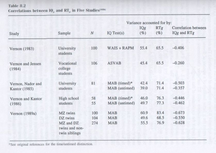
Vernon [48c] also found that when the g factor was partialed out of the WAIS + RAPM, none of the twelve subtests was significantly correlated with RTg. Interestingly, the RAPM, a nontimed test that shares no face content in common with any of the RT tests, has the largest g loading of any of the psychometric tests and also has the largest correlation with RTg. In contrast, Digit Symbol, which is the least complex and the most speeded of all the WAIS subtests, has the smallest g loading and also the smallest correlation with RTg. […]
Smith and Stanley [49a] correlated scores on eight psychometric tests separately with the RTs and RTSDs from the 2, 4, and 8 button conditions (1, 2, and 3 bits, respectively) of the Hick paradigm. The correlation coefficients constitute the column vector VRT (or VRTSD). The g loadings of the eight psychometric tests constitute the column vector Vg. For RT, the Vg x VRT correlations (r) for 1, 2, and 3 bits were -.765, -.160, and -.966, respectively (the 2-bits condition, with r = -.160, is obviously anomalous; the rank-order correlation is only -.270). For RTSD, or intraindividual variability in RT, the Vg x VRTSD correlations for 1, 2, and 3 bits were -.687, -.410, and -.772, respectively (again, the 2-bits condition, with r = -.410, seems anomalous, but here Spearman’s rank-order correlation rs is -.714.) The authors concluded, “It was clearly shown that the profile of the PT’s [psychometric tests’] g loadings could be well predicted from the RT-PT correlations for four of the RT measures. It can be concluded that RT tasks do measure general intelligence. Analysis of the errors in prediction suggested that the RTs may correlate more with fluid than crystallized intelligence” (p. 291).
An important point in the authors’ Table 1, but not mentioned by them, is seen in the correlations of all the RT and RTSD variables with g (the first principal component) and also with the next largest psychometric component (the bipolar verbal vs. spatial second principal component), which is perfectly uncorrelated with g and could be called a non-g factor. The average of all the g x RT and g x RTSD correlations is -.24 (p < .01), whereas the average of all the non-g x RT and non-g x RTSD correlations is +.02. This indicates that RT and RTSD are not correlated with any significant common factor in this psychometric battery other than g. In fact, I have not found an example of RT and RTSD being significantly correlated with any psychometric factor that is orthogonal to g.
Eleven ECTs (RTs and IT) given to seventy-three Navy recruits were used in a multiple correlation (R) to predict scores on each of the ten subtests of the Armed Services Vocational Aptitude Battery (ASVAB), the Raven Matrices (Advanced), and g factor scores derived from the ASVAB. [49b] The individual Rs ranged from .61 (for g factor scores) to .29 (for both Numerical Operations and Coding, the two most speeded tests in the ASVAB battery). The thirty-six-item Raven Matrices, with a forty-minute time limit, had the second largest correlation (R = .55). The correlation between the column vector of the twelve variables’ g loadings and the vector of the variables’ multiple Rs with the ECTs is r = .78.
The g loadings of RTs on various ECTs are clearly related to the complexity of the cognitive operations they call for. The mean RT of each of eight different ECTs in a sample of 106 vocational college students was used as an objective index of each ECT’s cognitive demand. The mean RTs of the eight ECTs ranged from 355 msec to 1,400 msec. The students also took the ASVAB, from which the g factor was extracted. The correlation between the eight RT means (on the ECTs) and the ECT’s correlations with g factor scores (from the ASVAB) is r = -.98 (rs = -.93), as shown in Figure 8.6.

A composite speed measure (based on RT, IT, and the Coding speed subtest of the WAIS) was obtained from 102 elderly persons (aged fifty-four to eighty-five). [49d] Partial correlations (with age partialed out) were obtained between this speed measure and each of eleven diverse psychometric tests. The vector of these correlations and the vector of the tests’ g loadings are correlated r = .95, rs = .72 (p < .01).
BLIND ALLEY EXPLANATIONS OF THE RT-g RELATIONSHIP
Motivation, Effort, Drive, and Arousal. Some psychologists have invoked this class of variables to explain the RT-g correlation and even g itself. The idea is that individual differences in performance on both psychometric tests and ECTs reflect mostly individual differences in subjects’ motivation and effort expended in the test situation. According to this theory, higher-scoring subjects are simply those who are more highly motivated to perform well. This explanation, though plausible, is contradicted by the evidence.
First, much is known empirically about the effects of these variables on cognitive performance, and the general principles derived from all this evidence appear to make this class of motivational variables an exceedingly weak prospect as an explanation of either g or the RT-g correlation. The Yerkes-Dodson law is most pertinent here. This is the well-established empirical generalization that the optimal level of motivation or drive (D) for learning or performance of a task is inversely related to the degree of complexity of the task; that is, a lower level of D is more advantageous for the performance of more complex tasks. In this respect, D is just the opposite of g. The g loading of tasks increases with task complexity, and persons who score highest in the most g-loaded tests are more successful in dealing with complexity. This is inconsistent with what is known about the effects of D on the performance of simple and complex tasks.
If individual differences in g were primarily the result of individual differences in D, we should expect, in accord with the Yerkes-Dodson law, that simple RT should be more correlated with g than two-choice RT, which should be more correlated with g than Odd-Man-Out RT. But in fact the correlations go in the opposite direction. Another point: The very low correlation between individual differences in RT and MT (movement time), and the fact that in factor analyses RT and MT have their salient loadings on different factors, would be impossible to explain by the motivational hypothesis without invoking the additional implausible ad hoc hypothesis that individual differences in motivation differentially affect RT and MT. As noted previously, RT is highly sensitive to differences in the complexity or information load of the reaction stimulus, while MT scarcely varies with task complexity. Despite this, subjects perceive RT and MT not as separately measured acts, but as a single ballistic response. It is most unlikely that a motivational effect would shift during the brief unperceived RT-MT interval.
The assessment of drive level and its attendant effort is not a function of subjective reports or of the experimenter’s merely assuming the effectiveness of manipulating subjects’ level of motivation by instructions or incentives. Drive level is reflected in objectively measurable physiological variables mediated by the autonomic nervous system. One such autonomic indicator of increased drive or arousal is pupillary dilation.
Pupillary diameter can be continuously and precisely measured and recorded by a television pupillometer while the subject is attending to a task displayed on a screen. This technique was used to investigate changes in effort as subjects were given relatively simple tasks (mental multiplication problems) that differed in complexity and difficulty. [51a] The subjects were two groups of university students; they had been selected for either relatively high or relatively low SAT scores, and the score distributions of the two groups were nonoverlapping on an independent IQ test. The whole ETC procedure was conducted automatically by computer; subjects responded on a microswitch keyboard. Here are the main findings: (1) pupillary dilation was directly related to level of problem difficulty (indexed both by the objective complexity of the problem and by the percentage of subjects giving the correct answer), and (2) subjects with higher scores on the psychometric tests showed less pupillary dilation at any given level of difficulty. The UCLA investigators, Sylvia Ahern and Jackson Beatty, concluded: “These results help to clarify the biological basis of psychometrically-defined intelligence. They suggest that more intelligent individuals do not solve a tractable cognitive problem by bringing increased activation, ‘mental energy’ or ‘mental effort’ to bear. On the contrary, these individuals show less task-induced activation in solving a problem of a given level of difficulty. This suggests that individuals differing in intelligence must also differ in the efficiency of those brain processes which mediate the particular cognitive task” (p. 1292).
Another study [51b] in this vein, based on 109 university students, measured two autonomic effects of increased motivation (heart rate and skin conductance) as well as a self-report questionnaire about the student’s subjective level of motivation and effort. The purpose was to determine if increasing motivation by a monetary incentive ($20) would improve performance on three computerized ECTs or affect the ECTs’ correlations with a composite score based on two highly g-loaded tests (Raven and Otis-Lennon IQ). Subjects were randomly assigned to either the incentive or the no-incentive conditions. Each subject was tested in two sessions; only those in the incentive group were offered $20 if they could improve their performance from the first to the second session. The incentive group reported a significantly (p < .01) higher level of motivation and effort than was reported by the no-incentive group. But the physiological indices of arousal recorded during the testing showed no significant effect of the incentive motivation. Processing speed (RT or IT) was not significantly affected by the incentive condition on any of the ECTs, although on a composite measure based on all three ECTs, the incentive group showed a small, but significant (p < .05) improvement from the first to the second session, as compared to the no-incentive group. The correlation of the combined ECTs with the composite IQ averaged .345 for the no-incentive condition and .305 for the incentive condition (a nonsignificant difference). Although both groups showed a significant practice effect (improvement) from the first to the second session on each ECT, the average ECT x IQ correlation was not affected. The authors concluded, “In no case . . . did incentives affect the overall IQ-performance correlation for the tests used in the battery. These results support the view that correlations between information processing scores and intelligence reflect common mental capacities, rather than some affective variable such as motivation” [51b] (p. 25).
NOTES
37. Two methods for combining RTs have been used: multiple regression and simple summation. In multiple regression, a different weight is given to each of the RT variables before they are summed for each subject; the weights (obtained by multiple regression analysis) are such as to maximize the correlation (now called a multiple correlation, R) between the weighted sum of the several RT variables and IQ (or whatever is the criterion or dependent variable). When the sample size is very large and the number of predictor variables (also called independent variables) is small, there is very little bias in the multiple R. (R is always biased upward.) The smaller the subject sample size and the larger the number of predictor variables, the more that the true R is overestimated. On the other hand, there is no such bias (or “capitalization on chance”) in a simple sum of the predictor variables, although the simple sum will not yield quite as large a correlation (r) as the multiple R. In most studies using multiple R, however, the R is corrected for bias. When the RTs from different ECTs have significantly different means, their combination in effect gives differential weights to the various ECTs. This may or may not be desirable, depending on the researcher’s purpose and the nature of the hypothesis being tested. When it is not considered desirable, it is preferable either to use multiple regression analysis to obtain the multiple R, or to assign unit weights to the RTs of the various ECTs. This is done by transforming all of the RTs (separately for each ECT) to standardized (z) scores and averaging these to obtain each subject’s unit-weighted RT z score.
Chapter 9
The Practical Validity of g
What exactly does a validity coefficient, rxc, tell us in quantitative terms? There are several possible answers, [2] but probably the simplest is this: When test scores are expressed in standardized form (zx) and the criterion measures are expressed in standardized form (zc), then, if an individual’s standardized score on a test is zxi, the individual’s predicted performance on the criterion is zci – rxc x zxi. For example, if a person scores two standard deviations above the group mean on the test (i.e., zxi = +2) and the test’s validity coefficient is +.50 (i.e., rxc = +.50), the person’s predicted performance on the criterion would be one standard deviation above the group mean (i.e., zci = rxc x zxi = +.50 x 2 = +1).
SCHOLASTIC ACHIEVEMENT
The evidence for the validity of IQ in predicting educational variables is so vast and has been reviewed so extensively elsewhere [11] that there is no need to review it in detail here. The median validity coefficient of IQ for educational variables is about +.50, but the spread of validity coefficients is considerable, ranging from close to zero up to about .85. Most of the variability in validity coefficients is due to differences in the range of ability in the particular groups being tested. The less the variability of IQ in a given group, of course, the lower is the correlation ceiling that the IQ is likely to have with any criterion variable. Hence we see an appreciable decrease in the average validity coefficient for each rung of the educational ladder from kindergarten to graduate or professional school. Several rungs on the educational ladder are the main junctures for either dropping out or continuing in school.
The correlation of IQ with grades and achievement test scores is highest (.60 to .70) in elementary school, which includes virtually the entire child population and hence the full range of mental ability. At each more advanced educational level, more and more pupils from the lower end of the IQ distribution drop out, thereby restricting the range of IQs. The average validity coefficients decrease accordingly: high school (.50 to .60), college (.40 to .50), graduate school (.30 to .40). All of these are quite high, as validity coefficients go, but they permit far less than accurate prediction of a specific individual. (The standard error of estimate is quite large for validity coefficients in this range.)
Achievement test scores are more highly correlated with IQ than are grades, probably because grades are more influenced by the teacher’s idiosyncratic perceptions of the child’s apparent effort, personality, docility, deportment, gender, and the like. For example, teachers tend, on average, to give higher course grades to girls than to boys, although the boys and the girls scarcely differ on objective achievement tests.
Even when pupils’ school grades are averaged over a number of years, so that different teachers’ idiosyncratic variability in grading is averaged out, the correlation between grades and IQ is still far from perfect. A strong test of the overall relationship between IQ and course grades was provided in a study [12] based on longitudinal data from the Berkeley Growth Study. A general factor (and individual factor scores) was obtained from pupils’ teacher-assigned grades in arithmetic, English, and social studies in grades one through ten. Also, the general factor (and factor scores) was extracted from the matrix of intercorrelations of Stanford-Binet IQs obtained from the same pupils on six occasions at one- to two-year intervals between grades one and ten. Thus we have here highly stable measures of both school grades and IQs, with each individual’s year-to-year fluctuations in IQ and teachers’ grades averaged out in the general factor scores for IQ and for grades.
The correlation between the general factor for grades and the general factor for Stanford-Binet IQ was +.69. Corrected for attenuation, the correlation is +.75. This corrected correlation indicates that pupils’ grades in academic subjects, although highly correlated with IQ, also reflect consistent sources of variance that are independent of IQ. The difficulty in studying or measuring the sources of variance in school grades that are not accounted for by IQ is that they seem to consist of a great many small (but relatively stable) sources of variance (personality traits, idiosyncratic traits, study habits, interests, drive, etc.) rather than just a few large, measurable traits. This is probably why attempts to improve the prediction of scholastic performance by including personality scales along with cognitive tests have shown little promise of raising predictive validity appreciably above that attributable to IQ alone. In the noncognitive realm, no general factor, or any combination of broad group factors, has been discovered that appreciably increases the predictive validity over and above the prediction from IQ alone.
Although IQ tests are highly g loaded, they also measure other factors in addition to g, such as verbal and numerical abilities. It is of interest, then, to ask how much the reported validity of IQ for predicting scholastic success can be attributed to g and how much to other factors independent of g.
The psychometrician Robert L. Thorndike [13] analyzed data specifically to answer this question. He concluded that 80 to 90 percent of the predictable variance in scholastic performance is accounted for by g, with 10 to 20 percent of the variance predicted by other factors measured by the IQ or other tests. This should not be surprising, since highly g-loaded tests that contain no verbal or numerical factors or information content that resembles anything taught in school (the Raven matrices is a good example) are only slightly less correlated with various measures of scholastic performance than are the standard IQ and scholastic aptitude tests, which typically include some scholastic content. Clearly the predictive validity of g does not depend on the test’s containing material that children are taught in school or at home. Pupils’ grades in different academic subjects share a substantial common factor that is largely g. [14]
The reason that IQ tests predict academic achievement better than any other measurable variable is that school learning itself is g-demanding. Pupils must continually grasp “relations and correlates” as new material is introduced, and they must transfer previously learned knowledge and skills to the learning of new material. These cognitive activities, when specifically investigated, are found to be heavily g loaded. It has also been found that various school subjects differ in their g demands. Mathematics and written composition, for example, are more g-demanding than arithmetic computation and spelling. Reading comprehension is so g loaded and also so crucial in the educational process as to warrant a separate section (p. 280).
The number of years of formal education that a person acquires is a relatively crude measure of educational attainment. It is quite highly correlated with IQ, typically between +.60 and +.70. [15] This correlation cannot be explained as entirely the result of more education causing higher IQ. A substantial correlation exists even if the IQ is measured at an age when all persons have had the same number of years of schooling. Validity coefficients in the range of .40 to .50 are found between IQ at age seven and amount of education completed by age 40. [16]
Equally important is the fact that the correlation between IQ and years of education is also a within-family correlation. A within-family correlation (explained in Chapter 6, pp. 139) cannot be the result of differences in social class or other family background factors that siblings share in common. This is evident from a study [17] in which g factor scores (derived from the first principal component of fifteen diverse mental tests) were obtained for adult full siblings (reared together). The difference between the siblings’ g factor scores and the difference in their number of years of education was +.50 for brothers, +.17 for sisters, and +.34 for brother-sister pairs. (Similar correlations were found for siblings’ differences in g and the differences in their occupational status.)
There is also a between-families component of the correlation between IQ and years of education associated with socioeconomic status (SES). More children at a given IQ level from high-SES families tend to be “overeducated” (i.e., are more likely to enter college) as compared with middle-SES and especially with low-SES children, who are less apt to enter college, given the same IQ as middle- and high-SES children.
THE VALIDITY OF g IN THE WORLD OF WORK
VALIDITY OF g FOR PREDICTING SUCCESS IN JOB TRAINING
Incremental Validity of Non-g Variance. … A study [24b] of the incremental validity of non-g (i.e., all sources of variance in the ten ASVAB subtests remaining after g has been removed) was based on 78,049 airmen in eighty-nine technical job training courses. The g factor scores had an average validity coefficient of +.76 (corrected for restriction of range due to prior use of the test for selection); the non-g portion of the ASVAB variance had an average predictive validity of +.02. The highest non-g validity for any of the eighty-nine jobs was +.10. Non-g had no significant validity for one-third of the jobs. Moreover, the relation between g and training success was practically the same for all jobs. When an overall average prediction equation for all eighty-nine jobs was compared against using a unique optimal prediction equation for each job, the total loss in predictive accuracy was less than one-half of 1 percent.
In the same study, the average g validity was lower (+.33) for actual performance measures than for course grades or a measure of job knowledge, but it was still appreciably higher than the corresponding average non-g validity, which was only +.05.
A study [24c] based on 1,400 navigator trainees and 4,000 pilot trainees used the sixteen subtests of the AFOQT to predict success in achieving a number of training criteria measured in actual performance of the required skills at the end of training. The g score validity (cross validated, range corrected) for the composite criteria was +.482 for navigators and +.398 for pilots. The corresponding incremental non-g validity coefficients were +.020 and +.084, respectively. Again, g proved to be the chief factor responsible for the AFOQT’s predictive validity.
The very small predictive validity of the ASVAB’s non-g component, it might be surmised, could result if each of the subtests measured scarcely anything other than g, despite the subtests’ quite different knowledge content. Empirically, however, this is clearly not the case. The g factor accounts for only 40 to 60 percent (depending on the range of ability in various samples) of the total variance of the ten ASVAB subtests. The remaining variance comprises group factors, test specificity, and measurement error (about 10 to 15 percent). Therefore, theoretically there is enough reliable non-g variance (about 30 to 50 percent) in the ASVAB for it to have an incremental validity almost as high as that for g.
Ratings based on structured interviews (which systematically assess subject attributes including educational background, self-confidence and leadership, flying motivation) were also found to have significant predictive validity for success in pilot training. [26] However, when the interview ratings were included in a multiple correlation along with the ASVAB to predict training success, the interview ratings proved to have no incremental validity over the ASVAB score. This finding indicates that whatever predictive validity the interview had was due to its overlapping variance with the predictive component of the ability factors tapped by the ASVAB, which is largely g.
VALIDITY OF g FOR PREDICTING JOB PERFORMANCE
Incremental Validity of Spatial and Psychomotor Aptitudes. … Major efforts to discover other psychometric variables that add appreciable increments over and above g to predictive validity for “core job performance” have not proved fruitful. [32] Of course there are many other aspects of success in life besides g or spatial and psychomotor factors, such as physical and mental energy level, effort, conscientiousness, dependability, personal integrity, emotional stability, self-discipline, leadership, and creativity. These characteristics, however, fall into the personality domain and can be assessed to some extent by personality inventories. A person’s interests have little incremental validity over g or other cognitive abilities, largely because a person’s interests are to some degree related to the person’s abilities. People generally do not develop an interest in subjects or activities requiring a level of cognitive complexity that overtaxes their level of g. Specialized talents, when highly developed, may be crucial for success in certain fields, such as music, art, and creative writing. The individual’s level of g, however, is an important threshold variable for the socially and economically significant expression of such talents. Probably very few, if any, successful professionals in these fields have a below-average IQ.
Linearity of Regression. The regression line, in terms of validity, is the line that best fits the relationship between the predicted criterion and the predictor test. In nearly all studies of the predictive validity of highly g-loaded tests, this regression line is linear (i.e., a straight line). This is illustrated, for example, in Figure 9.2, from a study where the Scholastic Aptitude Test (SAT) was used to predict college grade-point average (GPA) for students just entering college. The regression line per se is not shown in this graph, but the mean GPAs at equal intervals on the scale of SAT scores all fall on a single straight line, from the lowest possible SAT score (200) to the highest possible score (800). In other words, the regression of the criterion measure (GPA) on the predictor measure (SAT score) is linear throughout the entire range of GPAs and SAT scores. A similar picture emerges in hundreds of studies of the prediction of training success and job performance with various g-loaded tests. [34ab]

One of the mistaken beliefs about the predictive validity of IQ (and other g-loaded tests) is that beyond a certain threshold level, g has no practical validity, and individuals who score at different levels above the threshold will be effectively equivalent in criterion performance. This is another way of saying that the linear regression of the criterion on g does not hold above some point on the scale of g and beyond this point g-level is irrelevant. This belief is probably false. I have not found any study in which it has been demonstrated, except where there is an artificial ceiling on the criterion measure.
This is not to deny that as variance in g is decreased (owing to restriction of range in highly g-selected groups), other ability and personality factors that were not initially selected may gain in relative importance. But studies have shown that the linearity of the relation between g and performance criteria is maintained throughout the full range of g for all but the least complex performance criteria. Individual differences in IQ, even within groups in which all individuals are above the ninety-ninth percentile (that is, IQ > 140), are significantly correlated with differences in a variety of achievement criteria such as earning a college degree, intellectual level of college attended, honors won, college GPA, attending graduate school, and intensity of involvement with math and science. Since these are statistical trends to which there are many exceptions, prediction based on a g measure for a given individual is only probabilistic, with a wide margin of error. When individuals of a given level of g are aggregated, however, and there are several such aggregate groups, each at a different level of g, the correlation between the group means on g and the group means on the criterion measure approaches unity. [34c] Since many idiosyncratic subject variables are averaged out in the group means, the linear relationship of the criterion measure to g is clearly revealed.
Effect of Job Experience on Predictive Validity. There is no argument that job knowledge and performance skills increase with actual experience on the job. But it is a common misconception that the correlation between g-loaded test scores and job performance measures washes out after people have gained a certain base level of job experience. The idea here seems to be that learning the knowledge and skills needed to do the job is the most important thing and that once these are acquired through experience on the job, individual differences in whatever was measured by the selection test (mostly g) quickly become irrelevant.
Large-scale studies have proven that this notion is false. Job knowledge is the strongest predictor of work-sample performance, and the rate of acquisition and the asymptotic level of job knowledge gained through experience are both positively related to g. For jobs of moderate complexity, periodic assessments of job knowledge, work samples, and supervisor ratings, after four months to five years of experience on the job, show no systematic decrease in the predictive validity of g. [35] Five years of experience is simply the limit that has been tested to date, but there is no evidence to suggest that performance levels would be unrelated to g at any point in time beyond that limit. For jobs of greater complexity and autonomy, it is likely that individual differences in g would be reflected increasingly in performance with increasing experience.
OCCUPATIONAL LEVEL AS A FUNCTION OF g
Another way to demonstrate the overall relative magnitude of g differences between occupations is by analysis of variance. I have performed this analysis on all 444 occupational titles used by the U.S. Employment Service. The General Aptitude Test Battery (GATB) Manual presents the mean and standard deviation of GATB G-scores for large samples of each of the 444 different occupations. An analysis of variance performed on these data shows that 47 percent of the total G-score variance is between occupations (i.e., differences between the mean G-scores of the various occupations) and 53 percent of the variance is within occupations (i.e., differences between the G-scores of individuals within each occupation). Since about 10 percent of the within-occupations variance is attributable to measurement error, the true within-occupations variance constitutes only 43 percent of the total G-score variance. From these figures one can compute [39] the true-score correlation (based on individuals, not group means) between occupations and G-scores. It is .72, which closely agrees with the average correlation of .70 found in other studies in which individual IQs were directly correlated with the mean rank of people’s subjective ranking of occupations. The correlation of individuals’ IQs with occupational rank increases with age, ranging from about .50 for young persons to about .70 for middle-aged and older persons, whose career lines by then are well established.
The relation of IQ to occupational level is not at all caused by differences in individuals’ IQs being determined by the differences in amount of education or Ihe particular intellectual demands associated with different occupations. This is proved by the fact that IQ, even when measured in childhood, is correlated about .70 with occupational level in later adulthood.
NOTES
2. Another way of conceptualizing the meaning of a validity coefficient (rxc) is in terms of the following formula:
rxc = (T – R) / (P – R),
where T is the average level of performance on the criterion for persons selected with the test, R is the mean level of criterion performance for persons selected at random, and P is the mean criterion performance for perfectly selected persons, as if rxc = 1. Hence rxc is a direct measure of the proportional gain in the mean criterion performance that results from the use of the test for selection as compared to what the mean level of criterion performance would be with random selection. In other words, the validity coefficient is a direct indicator of the effectiveness of the test’s predictive accuracy, such that, for example, a validity coefficient of .50 provides just half as accurate prediction as a validity coefficient of 1.00, which indicates perfect prediction. Even a quite modest validity coefficient has considerable practical value when a great many binary (i.e., yes-no, pass-fail, win-lose) decisions are made. For example, the casino at Monte Carlo reaps large sums of money every day from its roulette games, because of course the house always has better odds for not losing than the gamblers have for winning, yet the house advantage is, in fact, equivalent to a predictive validity coefficient of only +.027! The practical value of a validity coefficient of +.27, therefore, is certainly not of negligible value where a large number of selection decisions must be made.
14. A factor analysis of pupils’ grades in six academic subjects yielded a general factor accounting for 58 percent of the total variance in grades, with factor loadings averaging .76 and ranging from .65 to .86. I performed this principal factor analysis on the correlation matrix given in an article by Rushton & Endler, 1977, p. 301. The correlations between six academic subjects (English, spelling, mathematics, geography, history, and science) ranged from .25 to .86, with a mean correlation of .56, for ninety-one pupils, aged ten to twelve. Besides the large common factor (i.e., the 1st PF) there was only one other factor with an eigenvalue > 1. It accounted for 9% of the total variance.
25. I have computed the correlation between the g vector and the vector of validity coefficients (corrected for restriction of range and controlling reliability) of the ten ASVAB subtests, using data reported in three other Air Force studies [24c,d] of navigator and pilot trainees, and the combined samples from 150 other different technical training schools. (A large part of these samples are included in the other reports described in the text.) The total N = 90,548. The N-weighted mean of the correlation between the vector of ASVAB subtests’ g loadings and the vector of the ASVAB subtests’ validity coefficients (averaged across schools) was +.95. All these results, taken together, leave no doubt that g is the chief active ingredient in ASVAB’s predictive validity for training success.
31. Ree and Carretta (1994) performed a confirmatory hierarchical factor analysis of four highly g-loaded subtests of the ASVAB along with eight psychomotor tests used in selection for pilot training in the Air Force (e.g., two-hand coordination in pursuit tracking, complex coordination, time-sharing tracking and monitoring, vertical and horizontal tracking). The best-fitting hierarchical factor model showed five first-order factors, a second-order psychomotor factor (common to all the psychomotor tests), and a g factor common to all of the tests, both cognitive and psychomotor. The g accounted for 39% of the variance in the whole battery; the psychomotor factor accounted for 29%. The g loadings of the eight psychomotor variables ranged from +.22 to +.51, averaging +.34. But the most important finding in this study, from the standpoint of g theory, is the comparison of the four ASVAB subtests’ g loadings when factor analyzed along with the psychomotor tests compared against their g loadings when they are factor analyzed separately from the psychomotor tests. The two sets of g loadings were almost identical; the largest difference between them was .04. I have compared the g loadings obtained on the four ASVAB subtests when factor analyzed among the psychomotor tests (in the sample of Air Force pilot trainees) with the g loadings of the same four ASVAB subtests when factor analyzed among the whole ASVAB battery of ten subtests (using data from a representative sample of about 12,000 American youths). The average difference between these two sets of g loadings was .025, the largest difference being .030. These findings (like those of Thorndike, 1987) contradict the claim that tests’ g loadings are highly erratic and vary markedly depending on the particular collection of tests among which they are factor analyzed. The four ASVAB subtests showed only very slight fluctuations in g loadings when factor analyzed among such contrasting test batteries as the total battery of ASVAB paper-and-pencil tests or the battery of hands-on mechanical devices used for measuring motor abilities.
Chapter 10
Construct, Vehicles, and Measurements
Vehicles. Likewise, two test batteries with quite different item contents can each be a good vehicle of g. However, under certain conditions one test may be better than the other. In a group of persons who have had the same schooling, for example, scores on a test containing many items of scholastic knowledge could be as highly correlated with a hypothetical true g as scores on a test containing only nonverbal items with no dependence at all on scholastic content. But in a group of much more heterogeneous educational background, the two types of tests probably would not be equally good vehicles of g. […]
Mental Measurements. To have any meaning at all, a test has to be “normed” on a subject sample of some denned population. A raw score (X) then can be transformed to a standardized score (called a z score), which is expressed as a deviation from the mean of the norm group in units determined by the standard deviation of the raw scores (i.e., z = [X – mean]/SD). The distribution of raw scores can even be “normalized,” that is, made to fit the normal curve perfectly, first by rank-ordering the raw scores, then converting the ranks to percentile ranks, and finally assigning to each percentile rank the standard score (z) corresponding to the percentile of a normal deviate, that is, all values of z distributed as the normal, or Gaussian, curve. (The IQ scale, with mean = 100 and SD = 15, is simply 100 + 15z.) An individual’s score on such a standardized or normalized scale only indicates that individual’s standing relative to the particular norm group. Most important: an individual’s test score (in either raw or standardized form) is not a measure of the quantity of the latent trait (e.g., g) per se possessed by that individual. […]
A rough analogy may help to make the essential point. Suppose that for some reason it was impossible to measure persons’ heights directly in the usual way, with a measuring stick. However, we still could accurately measure the length of the shadow cast by each person when the person is standing outdoors in the sunlight. Provided everyone’s shadow is measured at the same time of day, at the same day of the year, and at the same latitude on the earth’s surface, the shadow measurements would show exactly the same correlations with persons’ weight, shoe size, suit or dress size, as if we had measured everyone directly with a yardstick; and the shadow measurements could be used to predict perfectly whether or not a given person had to stoop when walking through a door that is only 5½ -feet high. However, if one group of persons’ shadows were measured at 9:00 A.M. and another group’s at 10:00 A.M., the pooled measurements would show a much smaller correlation with weight and other factors than if they were all measured at the same time, date, and place, and the measurements would have poor validity for predicting which persons could walk through a 5½ -foot door without stooping. We would say, correctly, that these measurements are biased. In order to make them usefully accurate as predictors of a person’s weight and so forth, we would have to know the time the person’s shadow was measured and could then add or subtract a value that would adjust the measurement so as to make it commensurate with measurements obtained at some other specific time, date, and location. This procedure would permit the standardized shadow measurements of height, which in principle would be as good as the measurements obtained directly with a measuring stick.
Standardized IQs are somewhat analogous to the standardized shadow measurements of height, while the raw scores on IQ tests are more analogous to the raw measurements of the shadows themselves. If we naively remain unaware that the shadow measurements vary with the time of day, the day of the year, and the degrees of latitude, our raw measurements would prove practically worthless for comparing individuals or groups tested at different times, dates, or places. Correlations and predictions could be accurate only within each unique group of persons whose shadows were measured at the same time, date, and place. Since psychologists do not yet have the equivalent of a yardstick for measuring mental ability directly, their vehicles of mental measurement — IQ scores — are necessarily “shadow” measurements, as in our height analogy, albeit with amply demonstrated practical predictive validity and construct validity within certain temporal and cultural limits.
TEST-RETEST CHANGE IN SCORES
Since the observed score increments could just as well reflect gains in test specificity rather than in g or any other common factors, a further analysis is required. A principal components analysis of the mean practice gains over all test-retest intervals on each of the GATB aptitudes reveals two significant components (eigenvalues > 1) that together account for 78 percent of the variance. However, neither one bears any resemblance to the aptitudes’ g loadings (Spearman rank correlations of -.048 and -.024, respectively). This tells us that the common factors in the score increments are not related to the g factor of the GATB. Probably subtest specificity, rather than any common factors, is the main constituent reflected in the score increments due to a practice effect. This interpretation is consistent with the general finding that practice effects, or even gains from specific training, on a given test show remarkably little transfer to other tests. The inverse relationship between g loadings and practice effects, and the relative absence of g in the increments themselves, may explain the low external validity of the IQ gains that result from specific training in the various cognitive skills assumed to be measured by IQ tests. The training-induced gains in IQ scores fail to predict external criteria (e.g., scholastic achievement) to the degree that would be expected if the induced gain in IQ represented a true gain in g, rather than merely a gain in the test’s specificity.
“SPONTANEOUS” CHANGES IN IQ ARE MOSTLY IDIOSYNCRATIC CHANCE
Individuals’ IQs fluctuate over the age range from early childhood to maturity and from later maturity to old age and death. IQ is relatively unstable in early childhood, but from age two to age ten it becomes increasingly stable and more highly predictive of individuals’ IQs in early adulthood. The correlation between IQ at age 10 and at age 18 is between .70 and .80; IQ measured at successive ages beyond age 10 gradually approaches a correlation of .90 with IQ at age 18. [8] Much of the variability in mental growth rates from early childhood to maturity is genetically programmed, as shown by the fact that monozygotic twins have nearly identical mental growth curves, with the same spurts and plateaus, while dizygotic twins show less similar growth curves, with spurts and plateaus occurring at different ages. [9] The decreasing stability of IQ in old age is related to increasing individual differences in general health and physical fitness and probably inherited differences in the rate of mental decline. Developmental psychologists and psychometricians alike have puzzled over the occasionally large and seemingly spontaneous changes in some individuals’ IQs and the fact that IQ has proven so resistant to change by means of psychological and educational interventions. If the cause(s) of the seemingly spontaneous changes could be discovered, perhaps they then could be intentionally manipulated to produce desired changes in IQ.
The most thorough study [10] analyzing spontaneous IQ changes that I have found in the literature is based on a representative sample of 794 children who were tested on the Wechsler Intelligence Scale for Children (WISC-R) at ages 7, 9, 11, and 13. The correlations of IQ at every age with every other age range from .74 to .84, indicating some instability in the children’s relative standings on IQ from one testing time to another. The magnitude of changes, in IQ points, was rather normally distributed, with a mean near zero and a slight positive skew (i.e., more extreme upward than extreme downward changes). The mean intraindividual standard deviation of IQ over all four test occasions was 3.35 points. At each testing interval, about 10 percent of the sample changed more than fifteen IQ points. For the vast majority of children, the fluctuations in IQ were small enough to be accounted for by the unreliability of measurement, but the IQ changes shown by that 10 percent of the sample were too large to fall within the range of normally distributed measurement errors, given the reliability and standard error of measurement of the WISC-R. Concerning this group with real and marked IQ changes, the authors stated, “[T]his change is variable in its timing, idiosyncratic in its source and transient in its course” (p. 455).
In an attempt to discover possible causes of the larger than chance IQ changes, the 107 most erratic testees were compared against the 687 relatively stable members of the sample on a set of thirty-seven family and child characteristics that have been theoretically or empirically related to IQ (such as perinatal problems, central nervous system syndromes, impaired vision or audition, motor development, behavior problems, family size, maternal health, family relations, socioeconomic status, moving location, changing caretakers, and the like). Only three of the thirty-seven variables showed a significant difference (p < .05) between the erratic and stable groups in frequency of occurrence (mean address changes by age thirteen, percent boys, motor development score). Out of thirty-seven such comparisons, one should expect about two significant ones to occur by chance alone. Therefore, it is quite possible that the two groups did not really differ overall more than chance expectancy in the variables thought to influence mental development. Other variables were also examined, such as parental separation or remarriage, nervous system trauma or illness, emotional problems, and the like. But for every child for whom a life event was linked to a marked IQ change, it was possible to find several other children who had experienced the same life event but who showed no detectable effect on IQ. The authors suggested that “the causes of marked IQ change may be unique events that occur in the lives of individual children; ‘the slings and arrows of outrageous fortune’” (p. 489). Also, they concluded, “[W]e cannot yet predict in advance whether or not a child’s IQ will change in response to any perturbing event, no matter how strong” (p. 491). The IQ is described as “elastic” rather than “plastic,” because marked changes in the trajectory of a child’s mental development are typically followed later by a return to the initial trajectory for that child. The finding that the reliable change in IQ that does take place is idiosyncratic and not associated with any identifiable environmental change is entirely consistent with the finding, based on the correlation of mental growth curves of MZ and DZ twins, that the observed spurts and plateaus in mental growth, as indicated by IQ, are about as genetically determined as individual differences in IQ measured on any one occasion during middle childhood and adolescence. [9]
THE SECULAR INCREASE IN IQ
Secular Decline in Scholastic Achievement Scores. During the same period that IQ performance was rising, scores on tests of scholastic achievement were declining, at all age levels. These opposite trends seem paradoxical, because, for students who have had the same amount of schooling, individual differences in scholastic achievement are highly correlated with IQ. When various achievement tests and IQ tests are factor analyzed together, both kinds of tests are highly loaded on a large general factor that is clearly g. These results provide a striking example of how the level of highly g-loaded measurements is influenced by the vehicle through which g is expressed. When the g-loaded test is composed largely of nonscholastic items (e.g., matrices, figure analogies), the raw scores show a secular increase; when an equally g-loaded test is composed of scholastic items (e.g., reading comprehension, math) the raw scores show a secular decrease. Obviously, the true level of g cannot be changing in opposite directions at the same time. The difference in vehicles must account for the discrepancy. So the extent to which the level of g per se has been rising (or falling) over the past few decades remains problematic.
About three-fourths of the decline in the national mean Scholastic Aptitude Test (SAT) score, from 1952 to 1990, is due to the increasing percentage of high school students with college aspirations who take the SAT (rising from about 5 percent in 1952 to about 30 percent in 1968). The pool of applicants, in fact, became increasingly less selective between 1960 and 1985. But even after this decline in test scores due to the changing composition of the college-going population is accounted for, a real SAT score decrement remains. Its cause has been attributed to the “dumbing down” of the school curriculum and slackening attainments in the kinds of academic knowledge and cognitive skills tapped by the SAT, especially by students in the upper quartile. [22] The overall decline in SAT scores has been slightly larger than the gain in IQ scores; when both are expressed in terms of ΔIQ, they amount to about -5 for the SAT and +3 for IQ. (The SAT-Verbal score declined slightly more than SAT-Math.)
Broader Implications of the Secular Rise in IQ. … A definitive test of Flynn’s hypothesis with respect to contemporary race differences in IQ is simply to compare the external validity of IQ in each racial group. The comparison must be based, not on the validity coefficient (i.e., the correlation between IQ scores and the criterion measure), but on the regression of the criterion measure (e.g., actual job performance) on the IQ scores. This method cannot, of course, be used to test the “reality” of the difference between the present and past generations. But if Flynn’s belief that the intergenerational gain in IQ scores is a purely psychometric effect that does not reflect a gain in functional ability, or g, is correct, we would predict that the external validity of the IQ scores, assessed by comparing the intercepts and regression coefficients from subject samples separated by a generation or more (but tested at the same age), would reveal that IQ is biased against subjects from the earlier generation. If the IQs had increased in the later generation without reflecting a corresponding increase in functional ability, the IQ would markedly underpredict the performance of the earlier generation — that is, their actual criterion performance would exceed the level of performance attained by those of the later generation who obtained the same IQ. The IQ scores would clearly be functioning differently in the two groups. This is the clearest indication of a biased test — in fact, the condition described here constitutes the very definition of predictive bias. [40] If the test scores had the same meaning in both generations, then a given score (on average) should predict the same level of performance in both generations. If this is not the case (and it may well not be), the test is biased and does not permit valid comparisons of “real-life” ability levels across generations.
When this kind of analysis is applied to contemporary black and white groups, the regressions are the same for both groups; that is, blacks and whites with the same test scores perform at the same level on the criterion. Hence it has been concluded that the test scores are not biased; they have the same meaning for each racial group. In hundreds of validity studies, the occasional exceptions to this generalization consist of finding tests that overpredict the performance of blacks. That is, the black level of real-world criterion performance is, on average, below that of whites with the same test score. This discrepancy is usually attributable (correctly) to the imperfect reliability of the test scores (even when the reliability is exactly the same for both racial groups). When the regressions are corrected for attenuation (unreliability), a single regression line predicts individuals’ level of performance equally well for each group. [41] This would not happen if the mean difference between the groups’ test scores were “hollow” with respect to g (and whatever other factors contribute to the test’s external validity). The nonexistence of predictive bias for the same test scores obtained by blacks or whites is a strong refutation of Flynn’s supposition that the secular trend in test scores explains away the observed average racial differences in IQ (i.e., that there is no real difference in the level of functional ability between races.)
Chapter 11
Population Differences in g
BLACK AND WHITE IQ DISTRIBUTIONS: STATISTICAL SUMMARY
Mean and Standard Deviation. … This measure is known both as the sigma difference (σ diff) or as the effect size (d). This standardized scale permits direct comparisons of mean differences regardless of the original scale of measurement or the characteristic measured. A meta-analysis of 156 independent studies of the W-B difference, based on many different IQ tests given to American samples, yields an overall mean sigma difference of 1.08σ. The a differences have a SD of 0.36, which means that about two-thirds of the mean W-B differences in these 156 studies fall between 0.72σ and 1.44σ, or roughly equivalent to mean IQ differences between ten and twenty points, with an overall average difference of 16.2. [4]
The pernicious notion that IQ discriminates mainly along racial lines, however, is utterly false. This can be demonstrated most clearly in terms of a statistical method known as the analysis of variance. Table 11.1 shows this kind of analysis for IQ data obtained from equal-sized random samples of black and white children in California schools. Their parents’ social class (based on education and occupation) was rated on a ten-point scale.
In the first column in Table 11.1 the total variance of the entire data set is of course 100 percent and the percentage of total variance attributable to each of the sources [6] is then listed in the first column. We see that only 30 percent of the total variance is associated with differences between race and social class, whereas 65 percent of the true-score variance is completely unrelated to IQ differences between the races and social classes, and exists entirely within each racial and social class group. The single largest source of IQ variance in the whole population exists within families, that is, between full siblings reared together in the same family. The second largest source of variance exists between families of the same race and the same social class.
… the average difference between blacks and whites of the same social class is 12 IQ points. The average difference between full siblings (reared together) is 11 IQ points. Measurement error (i.e., the average difference between the same person tested on two occasions) is 4 IQ points. (By comparison, the average difference between persons picked at random from the total population is 17 IQ points.) Persons of different social class but of the same race differ, on average, only 6 points, more or less, depending on how far apart they are on the scale of socioeconomic status (SES). What is termed the interaction of race and social class (8 percent of the variance) results from the unequal IQ differences between blacks and whites across the spectrum of SES, as shown in Figure 11.2. […]
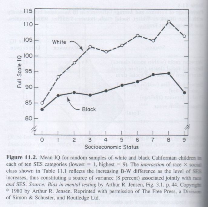
Constancy, Over Time. The mean W-B IQ difference has remained fairly constant at about 1σ for at least eighty years, with no clear trend upward or downward since the first large-scale testing of representative samples of blacks and whites in the United States. […]
Regional Variation. The mean IQ of blacks varies between different regions of the country, being generally lower in the Southeastern states, with an increasing gradient of IQ going toward the Northern and Western states. Whites show a similar, though less pronounced, regional gradient. As this gradient already appears in children’s IQ measured before school age, it is not entirely attributable to regional differences in the quality of schooling. The regional differences, some as much as ten to fifteen IQ points, are associated with earlier patterns of migration, the population densities in rural and urban areas, and the employment demands for different educational levels in various regions.
Age Variation. Black infants score higher than white infants on developmental scales that depend mainly on sensorimotor abilities. Scores on these infant scales have near-zero correlation with IQ at school age, because the IQ predominantly reflects cognitive rather than sensorimotor development. Between ages three and five years, which is before children normally enter school, the mean W-B IQ difference steadily increases. By five to six years of age, the mean difference is about 0.70σ (eleven IQ points), then approaches about 1σ during the elementary school years, remaining fairly constant until puberty, when it increases slightly and stabilizes at about 1.2σ. The latest (1986) Stanford-Binet IV norms show a W-B difference in prepubescent children that is almost five IQ points smaller than the W-B difference in postpubescent children. (The W-B difference is 0.80σ for ages 2 through 11 as compared with 1.10σ for ages 12 through 23.) This could constitute evidence that the mean W-B difference in the population is decreasing. Or it could simply be that the W-B difference increases from early to later childhood. The interpretation of this age effect on the size of the W-B mean difference remains uncertain in this instance, as it is based entirely on cross-sectional rather than longitudinal data. Both kinds of data are needed to settle the issue. The cause of variation in the mean IQ of different age groups all tested within the same year (a cross-sectional study) may not be the same as the cause of variation (if any) in mean IQ of the same group of individuals when tested at different ages (a longitudinal study).
Generality. The W-B difference in IQ is not confined to the United States, but is quite general and in the same direction, though of varying size, in every country in which representative samples of the white and black populations have been tested. The largest differences have been found in sub-Saharan Africa, averaging about 1.75σ in 11 studies. [7a,b] The largest difference between white and African groups (equated for schooling) is found on the Raven matrices (a nonverbal test of reasoning). In one large study the mean difference averaged about 2.0σ for Africans with no apparent European or Asian (East Indian) ancestry and about 1.1σ for Africans of mixed ancestry. [8] The East Indians in Africa averaged about 0.5σ below Europeans with the same years of schooling.
Studies in Britain have found that the mean IQ difference between the white and the West Indian (mainly African ancestry with some [unknown] degree of Caucasian admixture) populations is about the same as the W-B difference in the United States. [9] Recent immigrant East Indian children score, upon arrival in Britain, about as far below the British mean as do the West Indians, but, unlike the West Indians, the East Indians, after spending four years in British schools, score at about the same level as the indigenous white Britishers. A longitudinal study [10] of this phenomenon concluded, “The most striking result of the longitudinal IQ test results was the declining scores of the West Indians and the rising scores of the Indian children, in comparison to the non-minority children in the same schools. It appeared that the Indian children were acquiring the reasoning skills expected of children in the 8-12-year period, while the West Indians were not keeping pace in reasoning skills with most British children” (p. 40). The most recent British study [11] presents a somewhat different and more complex picture, to the effect that the most recent East Indian and Pakistani immigrants and those born in Britain within the last decade or so have scored less favorably on IQ tests and in scholastic performance than the earlier immigrants from the Indian subcontinent, although the Indian children were still on a par with the British in tests of reasoning and mathematics. It was only in the language area that they tested below the British children. Inexplicably, the Pakistanis performed conspicuously less well than the Indians. As these effects most likely reflect secular shifts in the particular self-selected segments of the home country’s population that emigrated to Britain, they would seem to be only of local interest and of questionable general significance. […]
IS THE W-B DIFFERENCE DUE TO CULTURE-BIASED TESTS?
Order of item difficulty is a completely internal indicator of bias. If the individual items in a test measure the same factor(s) in the black and white groups, then one should expect the rank order of item difficulty levels to be the same for both groups. If item #6 is harder (i.e., more difficult as indicated by the greater percentage of the sample who fail it) than item #5 in one group, item #6 should also be harder than item #5 in the other group. Thus we can rank the item difficulties in each group and look at the rank-order correlation between the two sets of ranks. This correlation can be compared with the rank-order correlation within each sample (or between two comparable sized samples each selected at random from the same racially homogeneous population). Item bias is indicated if the first correlation is significantly smaller than the second (meaning that the rank ordering of item difficulties is less alike in the two groups than it is in the same group). This method has been applied in many studies based on almost every widely used mental test, including the Wechsler scales and the Stanford-Binet. Invariably, the rank order of item difficulty for blacks and for whites is correlated over +.95 and is as high as the reliability of the rank order within each sample. Hence there is no evidence of bias by this internal criterion.
A stringent test of this criterion was performed [13] on a test intentionally composed of two types of items as judged by a group of psychologists: items judged to be either “culture-loaded” (C) or “noncultural” (NC). The mean W-B difference was actually smaller on the C group of items than on the NC items.
Here is the specific test for item bias: Relative item difficulty, separately for the black and the white groups, and separately for the C and NC items, was expressed for each of the items on an interval scale of difficulty known as the delta (Δ) scale. [14] The results are shown as a scatter diagram in Figure 11.4. The correlation (r) between the black and white Δ values for the 37 C items is +.96, for the 37 NC items r = +.95, and for all 74 items r = +.96. (The corresponding rank-order correlations are +.98, +.97, and +.97.) Hence, even in a test intentionally made up of items that are commonly expected to accentuate cultural item bias, no evidence of bias was found. […]

Unlike IQ itself, which is a standardized score with a mean of 100 and SD of fifteen for every age group, the raw scores of IQ tests increase steadily and almost linearly with age from early childhood up to about age fifteen years, after which they rapidly approach asymptote at a negatively accelerated rate of increase. The fact that the raw scores on each of the twelve subscales of the WISC-R tests do not show significant differences between blacks and whites in their correlations with age is presumptive evidence that the tests are measuring the same latent variables in both groups. [16] The regressions of scores on age, however, do differ in slope, with blacks showing a lower slope, indicating a slower rate of mental growth, with a lower asymptote.
That the correlation of IQ with either age-adjusted height or weight is not significantly different between very large samples of blacks and whites (approximately 12,000 in each sample) measured at ages four and seven years also suggests that IQ measures the same construct in both groups. [17] In the same samples there was a slight but significant W-B difference (W > B by about .05) in the correlation of IQ with age-adjusted head circumference. (The overall average correlations at ages four and seven years were .12 and .21, respectively.)
Two Types of Mental Retardation Mistaken as Test Bias. … In social and outdoor play activities, however, black children with IQ below seventy seldom appeared as other than quite normal youngsters — energetic, sociable, active, motorically well coordinated, and generally indistinguishable from their age-mates in regular clashes. But this was not so for as many of the white children with IQ below seventy. More of them were somehow “different” from their white age-mates in the regular classes. They appeared less competent in social interactions with their classmates and were motorically clumsy or awkward, or walked with a flat-looted gait. The retarded white children more often looked and acted generally retarded in their development than the black children of comparable IQ. From such observations, one gets the impression that the IQ tests are somehow biased against the black pupils and underestimate their true ability.
In most of the cognitive tasks of the classroom that call for conceptual learning and problem solving, however, black and white retarded children of the same IQ do not differ measurably either in classroom performance or on objective achievement tests. Trying out a variety of tests in these classes, I found one exception — tasks that depend only on rote learning and memorization through repetition. On these tasks, retarded black pupils, on average, performed significantly better than white pupils of the same IQ. [20]
The explanation for these differences cannot be that the IQ test is biased in its predictive validity for the children’s general scholastic learning, because predictive validity scarcely differs between black and white groups. Nor is the test biased according to any of the other standard criteria of bias (reviewed above). Rather, the explanation lies in the fact that IQ per se does not identify the cause of the child’s retardation (nor is it intended to do so).
There are two distinguishable types of mental retardation, usually referred to as endogenous and exogenous or, more commonly, as familial and organic. The lower tail (IQ < 70)) of the normal distribution of IQ in the population comprises both of these types of retardation.
In familial retardation there are no detectable causes of retardation other than the normal polygenic and microenvironmental sources of IQ variation that account for IQ differences throughout the entire range of IQ. Although persons with familial retardation are, on average, lower in IQ than their parents and siblings, they are no lower than would be expected for a trait with normal polygenic inheritance. For example, they score (on average) no lower in IQ compared with their first-order relatives than gifted children (above +2σ) score higher than their first-order relatives. Parent-child and sibling correlations for IQ are the same (about +.50) in the families of familial retardates as in the general population. In other words, the familial retarded are biologically normal individuals who deviate statistically from the population mean because of the same factors that cause IQ variation among all other biologically normal individuals in the population. Traits that are not associated with IQ in the general population do not distinguish the familial retarded from the rest of the biologically normal population. An analogy with stature, also a normally distributed polygenic trait, would be a physically strong, well-proportioned, well-nourished, healthy person of very short height. Such a person is neither a dwarf nor a midget, nor stunted by malnutrition or illness. (In the population distribution of adult male height, -2σ is about 5 ft., 2 in.).
Organic retardation, on the other hand, comprises over 350 identified etiologies, including specific chromosomal and genetic anomalies and environmental prenatal, perinatal, and postnatal brain damage due to disease or trauma that affects brain development. … The IQ of organically retarded children is scarcely correlated with the IQ of their first-order relatives, and they typically stand out as deviant in other ways as well. In the white population, for example, the full siblings of familial retarded persons have an average IQ of about ninety, whereas the average IQ of the siblings of organic retardates is close to the general population mean of 100.
Statistical studies of mental retardation based on the white population find that among all persons with IQ below seventy, between one-quarter and one-half are diagnosed as organic, and between one-half and three-quarters are diagnosed as familial. As some 2 to 3 percent of the white population falls below IQ seventy, the population percentage of organic retardates is at most one-half of 3 percent, or 1.5 percent of the population. Studies of the percentage of organic types of retardation in the black population are less conclusive, but they suggest that the percentage of organic retardation is at most only slightly higher than in the white population, probably about 2 percent. [21] However, based on the normal-curve statistics of the distribution of IQ in the black population, about 16 percent fall below IQ seventy. Assuming that organic retardation has a 2 percent incidence in the entire black population, then in classes for the retarded (i.e., IQ < 70) about 2%/16% = 12.5 percent of blacks would be organic as compared to about 1.5%/3% = 50 percent of whites — a white/black ratio of four to one.
VARIABILITY OF THE W-B DIFFERENCE: SPEARMAN’S HYPOTHESIS
[…] The W-B difference (in standard score units) was almost twice as large for backward digit span (BDS) as for forward digit span (FDS). Why should there be as large and consistent a difference between the W-B difference on FDS versus BDS? The contents of both tests are identical, namely, single random digits spoken by the examiner at the rate of one digit per second. In FDS, the examiner recites, say, four digits, and the subject is asked to repeat the digits in the same order. Then five digits are given, and so on, until the subject is unable to repeat all n digits correctly on two successive trials. The procedure for BDS is exactly the same, except that the subject is asked to repeat the series of digits in the reverse order to that presented. (The average adult can recall seven digits forward, five digits backward.)
Several studies [22] showed, in every age group, that the W-B difference on the FDS test is smaller (usually by about 0.5σ) than on the BDS test. Also, when black and white groups were matched on mental age (thus the blacks were chronologically older than the whites), the black and white means did not differ, either on FDS or on BDS. These results are not easily explained in terms of a qualitative cultural difference or some motivational factor. Rather, the results are most parsimoniously explained in terms of a difference in the black and white rates of development of whatever abilities enter into FDS and BDS. BDS obviously makes a greater demand on mental manipulation of the input in order to produce the correct output than does FDS. Hence BDS can be characterized as a more complex cognitive task than FDS. Further, a factor analysis of FDS and BDS scores obtained at five grade levels clearly showed (in separate analyses for blacks and whites) that two distinct factors are reflected in these tests, with the most salient loadings of FDS and of BDS found on different factors.
Is the g Factor the Same in Black and White Groups? … Over the seventeen studies, the congruence coefficient between the g factors extracted from the black and the white samples ranges from .976 to .999; the mean and median are both equal to .995. Clearly, we must conclude that factor analysis yields essentially the same g factor for both the black and the white samples on each of these seventeen different test batteries. In most cases, the residualized group factors (i.e., lower-order factors independent of g) show nearly as high a degree of black/white congruence, with congruence coefficients over .990 when samples are very large (which decreases the sampling error). In a study [28] of 212,238 white and 32,798 black applicants who took the seventeen diverse subtests of the U.S. Air Force Officer Qualifying Test, a hierarchical factor analysis yielded g and five first-order factors. The black/white congruence coefficients were +.99 for each of the factors. (The Pearson correlations between the vectors of factor loadings ranged between .97 and .99, and the groups did not differ in the average size of the g loadings.)
The g factor of a given battery also remains consistently the same factor across different age groups. Probably the best data that can be examined for this purpose are those based on the Kaufman Assessment Battery for Children (K-ABC), as this battery contains thirteen highly diverse tests representing at least three distinct factors besides g. Using the national standardization data to compare the g factor obtained in two age groups (ages 7 to 8 years versus 11 to 12.5 years), the g congruence coefficient for black children is .991; for white children, .998. (The black/white g congruence within each age group is at least .99.) The g factor (first principal component) accounts for about the same percentage of the total variance (averaging 58 percent) among the K-ABC subtest scores for different age groups (between 7 and 12.5 years) and for blacks and whites. [29] […]
For seventeen studies of young children (aged 3 to 6, averaging 5.2 years) published between the years 1922 and 1965, the mean W-B IQ difference on individually administered IQ tests was 10.76 (SD 8.0). The year of the study and the W-B IQ difference are correlated +.55, showing that the W-B difference for this age group has increased over time.
For thirty-three studies of elementary school children (aged 5 to 15, averaging 9.61 years) published between the years 1920 and 1964, the overall mean W-B IQ difference was 14.63 (SD 6.8). For thirty-one studies based on nonverbal group tests, the mean W-B IQ difference was 14.32 (SD 5.9). For 160 studies of elementary school children based on verbal group tests, the mean W-B difference was 14.51 (SD 7.9). For elementary school children, then, the average W-B difference on all three types of tests is 14.5 IQ points. The year of the study and the W-B IQ difference are correlated +.29, showing an increased B-W difference over time for this age group also.
IQ data obtained from students enrolled in high school are no longer very representative of the black and white populations at that age, because of the differing school dropout rates associated with IQ. The probability of a student’s dropping out of high school is negatively correlated with IQ, and blacks have had much higher dropout rates than whites [31] during the period covered by Shuey’s review. This should produce a decrease in the W-B IQ difference if measured for students actually in high school. In fact, 117 studies of high school students showed a mean W-B IQ difference of 10.40 (SD 6.4). A more representative estimate of the IQs of youths between ages eighteen and twenty-six can be obtained from the immense samples of enlisted men in the armed services during World War II. These subjects took the Army General Classification Test (AGCT), which is as highly correlated (r ≈ .80) with various IQ tests as the IQ tests are correlated with each other. The mean W-B difference on the AGCT was 1.25σ, which is equivalent to 18.7 IQ points. More recent data are provided by the national standardization of the 1986 Stanford-Binet IV, which shows a W-B difference of 1.13σ (or 17.4 IQ points) for youths twelve to twenty-three years of age. [32]
In summary, the cross-sectional data show an increasing mean W-B IQ difference from early childhood (about 0.7σ), to middle childhood (about 1σ), to adolescence and early maturity (about 1.2σ). The same data provide no evidence to indicate a decrease in the mean W-B difference in IQ over the last 20 years or so. [33] There is, however, considerable evidence of a significant decrease in the W-B difference on some scholastic achievement tests, largely due to educational gains by blacks — probably because of blacks’ increased attendance rates, years of schooling, and special services in recent decades. (See Chapter 14, Figure 14.2, p. 562.)
Tests of Spearman’s Hypothesis. … Figure 11.6 shows the scatter diagram for the correlation between the mean group difference (D in σ units) and the g loadings of 149 psychometric tests obtained in fifteen independent samples totaling 43,892 blacks and 243,009 whites. The correlation (with the effects of differences in tests’ reliability coefficients partialed out) is highly significant (t = 9.80, df = 146, p < .000). Hence there can be little doubt that Spearman’s hypothesis is borne out. Assiduous search of the literature has not turned up a single set of data with six or more diverse tests given to representative samples that contradicts Spearman’s hypothesis. [35]

A further validating feature of these data is revealed by the linear regression of the standardized W-B differences on the tests’ g loadings. (The regression equation for the W-B difference, shown in Figure 11.6, is D = 1.47g – .163). The regression line, which indicates the best estimate of the mean W-B difference on a test with a given g loading, shows that for a hypothetical test with zero g loading, the predicted mean group difference is slightly below zero (-.163σ), and for a hypothetical test with a g loading of unity (g = 1), the predicted mean group difference is 1.31σ. […]
Tests that rather consistently show a larger W-B difference (in favor of whites) than is predicted by their g loadings are those that, besides being loaded on g, are also loaded on a spatial visualization factor. Examples are tests such as paper folding, block counting, rotated figures, block design, object assembly, and mazes. When groups of blacks and whites are perfectly matched on the WISC-R Full Scale IQ (which is nearly equivalent to a g score), whites still exceed blacks, on average, by as much as ½σ on the most spatially loaded subtests. [34c,i] The tests that rather consistently show a smaller W-B difference than is predicted by the tests’ g loading (and, in fact, favor blacks) are those that are also loaded on a short-term memory (STM) factor. Examples are tests such as the Digit Span and Coding subtests of the WISC-R. When black and white groups are matched on Full Scale IQ, blacks exceed whites by as much as 0.62σ on Digit Span and 0.49σ on Coding, the two tests with the highest loadings on the STM factor. In the WISC-R Full Scale IQ, therefore, the whites’ average advantage on the spatial factor more or less balances the blacks’ advantage on the STM factor. Almost all of the remaining group difference on the test as a whole is therefore attributable to g.
Spearman’s Hypothesis with SES Controlled. Countless studies have shown that school-age children’s IQs are correlated with their parents’ socioeconomic status (SES), as determined mainly by their occupational and educational level. Most of the IQ/SES correlations fall in the range of .35 to .45. (This implies a similar degree of correlation between g and SES.) Several facts indicate that the causal direction of the IQ/SES correlation is largely from IQ to SES: Adoption studies show near-zero correlations between adoptees’ IQs and the SES of their adoptive parents; there is a virtual absence of between-families, or shared, environmental variance in IQ; and IQ is more highly correlated (about .70) with individuals’ own attained SES (as adults) than individuals’ IQs are correlated with their parents’ SES (about .40). In the simplest terms, with arrows indicating the direction of predominant causality,

Because blacks and whites differ, on average, in SES, it could be claimed that Spearman’s hypothesis simply reflects this fact, and nothing more. The IQ/SES relationship, of course, makes it practically inevitable that (within either racial group) the vector of subtests’ correlations with SES would be correlated with the vector of subtests’ g loadings. In fact, this correlation, based on thirteen subtests of the WISC-R standardization data, is +.84 for whites and +.39 for blacks. [34c] It appears that blacks are much less differentiated in IQ by SES than are whites, which is consistent with the picture in Figure 11.2 (p. 358) based on WISC-R data from an independent sample.
The possibility that Spearman’s hypothesis simply reflects the W-B difference in SES was studied with eighty-six matched pairs of black and white fourth- and fifth-graders from three schools. [34h] Each black child was matched with a white child on a five-point scale of SES, and also on age, school, and sex. Each child was individually administered the WISC-R (11 subtests) and the K-ABC (13 subtests). The test of Spearman’s hypothesis was based on the combined batteries, 24 subtests in all. A hierarchical (second-order) g factor was extracted from this battery and the vector of the 24 subtests’ g loadings was correlated with the vector of standardized mean W-B differences. The Pearson r is +.78, the Spearman rs is +.75 (p < .01), and the partial correlation (with the subtests’ reliability coefficients partialed out) is +.85. The scatter diagram is shown in Figure 11.8.

Spearman’s hypothesis is substantiated even more clearly by these data on SES-matched groups than by black and white groups that differ in SES. All the other studies that have substantiated Spearman’s hypothesis obviously cannot be explained in terms of SES. The SES-matched black and white groups in this study showed the following differences (W-B in σ units) on the orthogonalized factor scores derived from the twenty-four subtests: g .77σ, Verbal .20σ, Spatial .39σ, Memory .01σ. (In IQ units these differences are 12, 3, 6, and < 1, respectively.) The significant W-B differences on two of the group factors (Verbal and Spatial) independent of g is consistent with the weak form of Spearman’s hypothesis.
Spearman’s Hypothesis in Preschoolers. Only one study [34j] has reported a test of Spearman’s hypothesis based on preschoolers. These physically normal, healthy children, drawn from lower, lower-middle, and middle-class areas of Cleveland, were between the ages of 3.0 and 3.4 years. The thirty-three black and thirty-three white children were matched on age, sex, birth order, and mother’s education (which averaged 13.58 for the black mothers and 13.24 years for the white). The groups differed significantly in birth weight (B < W), but within each racial group the children’s birth weights were not significantly related to their IQs on the Stanford-Binet IV (SB-IV). Despite matching black and white children for maternal education, the children’s mean W-B IQ difference was 15.2 IQ points (in terms of the recent SB-IV norms) and 1.39σ in terms of the study group’s SD. Maternal education was significantly related to IQ independently of race; that is, maternal education and child’s IQ are correlated within each racial group.
The groups also differed significantly (B < W) on each of the eight subtests (vocabulary, comprehension, absurdities, pattern analysis, copying, quantitative, bead memory, memory for sentences). The rank-order correlation between the vector of the subtests’ disattenuated g loadings and the vector of the disattenuated mean W-B differences is rs = +.71 (significant beyond the .05 level), which strongly bears out Spearman’s hypothesis among three-year-olds.
Two other features of this study are also relevant to Spearman’s hypothesis: (1) The column vector of standardized mean W-B differences on each of the subtests is correlated rs = 0.00 with the column vector of the magnitudes of the standardized difference (averaged within groups) in the effect of maternal education on each subtest. [41] (2) The vector of the subtests’ g loadings is correlated rs = .26 (nonsignificant) with the vector of magnitudes of the effect of maternal education on the children’s performance on each subtest. In other words, there seems to be no relationship between the relative magnitudes of the W-B differences on these subtests and the effects of maternal education on each of the subtests, and no relationship between the subtests’ g loadings and the effects of maternal education. In accord with Spearman’s hypothesis, the subtests’ g loadings significantly predict the rank order of W-B differences. But the effect of maternal education on the subtests does not predict the rank order of the W-B differences on the subtests or the subtests’ g loadings.
SPEARMAN’S HYPOTHESIS TESTED WITH ELEMENTARY COGNITIVE TASKS
Having separate measurements of RT and MT is especially important in the study of group differences for two reasons: (1) As RT is more related to g than is MT, a composite of RT + MT attenuates any correlation with g; (2) as RT and MT represent different processes (cognitive and motor, respectively) group differences could go in opposite directions on each variable. If measured as a composite, their effects would cancel each other and obscure the detection of a difference between groups. In fact, there is some evidence for this kind of effect in studies of elementary school children, which show that on tasks more complex than simple RT (SRT), whites have shorter RT than blacks, on average, while blacks have shorter MT than whites. [47] Because this phenomenon does not appear in samples of blacks and whites as young adults, [48] it seems to reflect W-B differences in the rate of cognitive development and of motor development during childhood.
In general, mean W-B differences on various ECTs show effects similar to those found for individual differences within either group. For example, the WB difference increases with task complexity or difficulty when complexity is objectively measured by the average RT for each task in the combined groups.
In a study [49] based on black and white male students in a vocational college, the mean B-W difference in RT on each of eight ECTs of differing information processing complexity was significantly correlated with the mean RT of each task in the combined groups, as shown in Figure 11.9. Note that even the most difficult of these tasks had a mean RT of only 1.3 to 1.4 seconds. Also there was a high correlation (r = +.96, rs = +.88) between the complexity of the eight tasks (as measured by the mean RT for each task in the combined groups) and the tasks’ g loadings (i.e., their correlation with g factor scores derived from the ASVAB battery). The mean W-B difference was 0.7σ on psychometric g (derived from the ten ASVAB subtests) and 0.2σ on the general factor of the eight processing tasks. The group difference on the processing tasks was the same as the average difference between two individuals (of the same race) who differ by 0.7σ in psychometric g. The data of this study bear out the prediction of Spearman’s hypothesis: The B-W difference in RT on each of the eight processing tasks has a rank-order correlation with the tasks’ g loadings of rs = -.86 (p < .01).

An African Study. A study by Dutch psychologist Y. H. Poortinga [50] based on white and black African university students (both groups in South Africa) showed virtually no differences on either simple or two-choice RT to visual and auditory stimuli, but showed quite large and significant B-W differences, measured in standard deviation (a) units, on four-choice and eight-choice RT, as shown below (the mean RT differences are B minus W):

Although the four-choice and the eight-choice auditory RTs were significantly correlated (-.45 and -.38) with the highly g-loaded Raven’s Advanced Progressive Matrices (APM) for the white sample, there was no significant correlation for the black sample (probably because of the restricted range of scores). The study’s author noted that the APM was too difficult for the black students, whose average APM score was 2.2σ below that of the white students. (On two other psychometric tests the groups differed by 2.3σ and 1.5σ.)
The failure of these RT tasks to show significant correlations with highly g-loaded psychometric tests in the African sample could indicate either that the RTs do not reflect g in this group of African blacks or that these psychometric tests do not accurately measure g in this group. The fact that the three psychometric tests are substantially correlated with each other (.64, .73, and .59) indicates a good deal of common variance. But it could be that in the African sample the largest common factor is something other than the g factor [51] (which is the largest common factor in such tests for the white sample). As the average correlation between scores on highly g-loaded tests and eight-choice RT tasks is about .25 (based on several studies that do not include African blacks), and as the African W-B difference on the APM was 2.2σ, the predicted B-W difference on choice RT would be .30 x 2.2σ = 0.66σ, which is only about half as large as the mean difference actually found between the black and white students in Africa.
The Raven APM therefore greatly underpredicts the W-B difference in eight-choice RT. This could be because for this sample of African blacks the relation between RT and psychometric g is not the same as in the white samples studied. Poortinga suggests his findings were probably a result of using a test that was too difficult for this group of black students. The APM probably has too little variance and too serious a “floor effect” (i.e., a piling up of scores near the chance guessing level) to serve as an adequate measure of g in this African group. The mean and SD of the APM in the African sample were 9.2 and 5.66, respectively. On American norms, this corresponds to an IQ of 92 (SD = 6), but chance guessing on the APM produces a score equivalent to an IQ of 90. Thus the APM scores obtained by the nearly one-half of the black sample who scored below IQ 90 do not reflect reliable variance in g. The Standard Progressive Matrices (SPM), which was designed for the middle range of ability, would have been more suitable for the African sample than was the APM, which was designed for testing in the upper half of the distribution of g in the white European and North American populations. [52]
A Critical Test of Spearman’s Hypothesis. … Evidence of the reliability of the pattern of the ECT variables’ g loadings is the correlation between the vector of g loadings for blacks and the corresponding vector of g loadings for whites. Both the Pearson correlation and the rank-order correlation are +.85; the congruence coefficient is +.97. This shows that the ECT variables represent one and the same g for both the black and the white groups. Therefore, each variable’s g loadings could be averaged across the black and white groups, yielding a single vector of twelve g loadings.
The construct validity of the rank order of the ECT variables’ g loadings is shown by their correlation with the theoretically expected rank order of their loadings on psychometric g. The theoretical rank order of these ECT variables’ g loadings is based on a number of general principles derived from many previous studies (which, in fact, correspond to our everyday notions of how “complex” the tests are). [54] Figure 11.11 shows the rank-order correlation of rs = +.89 between the obtained g loadings (averaged over blacks and whites for each variable) and the theoretically expected g loadings. The fit between the theoretical and the obtained rank orders is quite good and is far beyond chance probability (p < .001).

As a test of Spearman’s hypothesis, then, this column vector of (average) g loadings for each of the twelve ECT variables was correlated with the vector of the twelve standardized mean B-W differences on each of the ECT variables. The Pearson r = +.81, the rank-order rs = +.79, p < .01. The rank-order correlation scatter diagram between the vector of g loadings and the vector of B-W differences is shown in Figure 11.12. It bears out Spearman’s hypothesis even more strongly than do most of the studies performed with conventional psychometric tests.

Spearman’s Hypothesis Tested with South Africans. The very same variables and apparatuses designed to be as much like those used in the previously described study were used by Lynn and Holmshaw [58] to test Spearman’s hypothesis on samples consisting of nine-year-old black schoolchildren in South Africa (N = 350) and white schoolchildren of comparable age in Britain (N = 239). The testing procedures were virtually identical to those in the American study based on children averaging about eleven years of age. Because of the difference in subjects’ ages in the South African and American studies, a direct comparison on the actual time measurements of RT and MT would not be relevant here. However, the Lynn and Holmshaw study showed much the same pattern of B-W differences (in σ units) across the twelve ECT variables as was found in Jensen’s American study, the main difference being in the size of the differences, which are generally much larger in the South African study. The South African blacks were markedly slower than the British whites in RT and also markedly faster in MT. But note that the same phenomenon was present in both studies; that is, whites outperformed blacks on the RT component of the task (which is correlated with g) while blacks outperformed whites on the MT component.
The greater B-W differences on the RT and RTSD components of the ECTs in the South African study is best explained by the fact that this group of South African blacks scored, on average, about 2σ below British (or South African) whites, while there is only about 1σ difference between American blacks and whites. [59] In the Lynn and Holmshaw study, the W-B difference on Raven’s Standard Progressive Matrices (SPM) was about 2.5σ. But we cannot be very confident of this value, because the SPM appeared to be too difficult for the African blacks. Their mean raw score on the SPM was only about three points above the chance guessing score, which casts doubt on the reliability and validity of the SPM as a measure of individual differences in g for this sample.
The questionable SPM scores for the South African blacks showed much lower correlations and a quite different pattern of correlations with the ECTs than were found in the white sample. Therefore, it is hardly surprising that the data of this study do not accord with Spearman’s hypothesis. A proper test of the hypothesis was not even possible, because the vector of the correlations between the ECTs and the SPM, which estimates the g loadings of the ECTs, showed too little congruence between blacks and whites to represent the same vector of factor loadings for the two groups in this study. (The congruence coefficient is only .45, which falls far below the generally accepted minimum value of .90 needed to claim that the factors are similar. The corresponding congruence coefficient in all of the other studies of Spearman’s hypothesis ranges from .98 to 1.00, with a mean of .995.)
However, it is noteworthy that the ECTs yielded meaningful data for the South African blacks. The vector of B-W differences on the twelve ECT variables does, in fact, conform to Spearman’s hypothesis when it is compared with the vector of g loadings based on the American data. (For a highly detailed analysis of the limitations of the statistical data reported in the Lynn and Holmshaw study, see Note 60.)
The ECT Variables in a Chinese-American Sample. Exactly the same tests and procedures as were used in the test of Spearman’s hypothesis based on black and white children in California were used in a parallel study of Chinese-American children and white children in elementary school (grades four through six). [61] Most of the Chinese-American children (some of them recent immigrants) were of considerably lower SES than most of the white children, yet the Chinese, on average, outscored the whites by a highly significant 0.32σ (equivalent to five IQ points) on the Raven SPM.
Although Spearman’s hypothesis was originally concerned only with W-B differences on psychometric tests, it is of interest to determine if the mean test-score differences between other groups show the same phenomenon. In the case of the Chinese-white comparison, the rank-order correlation of rs = +.01 obtained between the vector of the ECT variables’ g loadings and the vector of Chinese-white differences on each of the ECT variables is obviously not significantly greater than zero. The vector of the twelve ECT variables’ g loadings (i.e., their correlations with Raven’s SPM) had satisfactory congruence across the two racial groups (congruence coefficient = +.92), indicating that the ECT variables were similarly related to psychometric g in both groups. The Chinese had as fast or faster CRT and DRT than the whites, but had very markedly slower MT than whites on every task. The Chinese were slower than whites on SRT, probably because of its relatively large motor component compared to its cognitive, or g, component. It seemed likely that the motor aspect of RT was relatively larger than the cognitive part of RT for the Chinese children. This would attenuate the Chinese-white difference in speed of information processing as measured by RT. To test this conjecture, for every subject, SRT was subtracted from CRT and from DRT, thus ridding CRT and DRT of their motor component. The resulting scores showed the Chinese to be about 0.4σ faster than the whites in information-processing time, a slightly larger difference even than was found on Raven’s SPM. The Chinese-Americans were faster than the whites in information-processing time on CRT and DRT by twenty-seven and fifty-two milliseconds, respectively. These seemingly small differences in information-processing speed when brought to bear on much more complex tasks operating over considerable periods of time could result in quite noticeable differences in overall intellectual achievement.
The Math Verification Test in a Chinese-American Sample. In another study [62] the MVT was applied to samples of Chinese-American (N = 155) and non-Hispanic white pupils (N = 73) in regular classes of grades four through six. The whites scored 0.32σ below the Chinese-Americans on Raven’s SPM. All of the MVT procedures and variables were the same as in the study of blacks and whites.
All of the RT and RTSD variables had highly significant correlations with the SPM (average r = -.25, p < .001); none of the MT and MTSD variables was significantly correlated with the SPM (mean r = +.01). On RT and RTSD, the overall standardized mean white-Chinese difference was 0.34σ, about the same as the 0.32σ difference they showed on Raven’s SPM. (The actual overall mean RT for the whites was 1,480 msec; for the Chinese, 1,204 msec.) But note: The overall average white-Chinese difference on MT and MTSD was in the opposite direction, -0.19σ.
When the vector of the twelve MVT variables’ g loadings was correlated with the vector of the white-Chinese standardized mean differences on each of the MVT variables, the Pearson r = -.93 and the rank order rs = -.90 (p < .01). This indicates that the larger the MVT variable’s estimated g loading (i.e., its correlation with the SPM), the more the Chinese outperform the whites on the MVT. On this test, the whites compared with the Chinese in much the same way that the blacks compared with the whites in the previous study. It should be noted that these Chinese children were mostly of lower SES than the white children. The three racial groups — Chinese, white, and black — score in the same rank order both on the SPM and on untimed paper-and-pencil tests of mathematical problem solving.
NOTES
24. Both the Pearson r and Spearman’s rank-order correlation, rs, are suitable measures of the degree of relationship between the two vectors. It is most informative to report both; rs is much less affected by outliers that can spuriously inflate r. A statistical test of whether the obtained correlation differs significantly from zero should be based on rs rather than on r, because r is a parametric statistic for which the calculation of its standard error rests on the assumption of normality of the population distributions of each of the correlated variables. But there is no proper basis for assuming anything at all about the form of either the distribution of g loadings or the distribution of standardized mean W-B differences for the total “population” of all cognitive tests. In such a case, a nonparametric statistic is called for, as its standard error is not based on any assumption about the population distributions of the correlated variates. Spearman’s rs is such a nonparametric measure of correlation; its level of statistical significance is based simply on a permutation test, that is, the probability that the degree of agreement between the rank orders (from one to n) of the two sets of n variates would be as great as (or greater than) the value of the obtained rs in all possible permutations of the n ranks. (The total possible permutations of n different numbers is n!.) The test of significance of rs is always an exceedingly stringent statistical test of Spearman’s hypothesis, because the n (the number of different psychometric measures that can be feasibly administered to groups in any one study) is typically a rather small n. (The total range of n in all of the studies of Spearman’s hypothesis to date goes from six to seventy-four different psychometric tests.)
The fact that the test of significance of rs depends only on n (the number of measurements in each of the correlated vectors) does not mean that the number of subjects (N) in the study is unimportant. The larger the N, the smaller will be the standard error of the g loadings and the larger will be the standardized mean W-B differences, and hence the more reliable will be their vectors and so the more likely that there will be a significant correlation between the two vectors, if Spearman’s hypothesis is true.
26. Test unreliability must be considered because it has the effect of decreasing both the g loadings and the standardized mean W-B differences. If the various tests’ reliability coefficients differ significantly, being higher on some tests than on others, then, because they affect each test’s factor loading and standardized mean group difference to the same relative degree, a correlation between the vector of loadings and the vector of differences could be entirely an artifact of differences in the reliability of the various tests. On the other hand, if the vector of the tests’ reliability coefficients were negatively correlated with either the vector of factor loadings or the vector of mean differences, this fact could obscure or counteract the possibility of a significant correlation between the two vectors for which Spearman’s hypothesis predicts a positive correlation. Clearly, the vector of the tests’ reliability coefficients has to be dealt with to remove its potentially distorting effect on the test of Spearman’s hypothesis. (There would be no problem, of course, if the tests all had the same reliability.)
The two methods for controlling for the effect of the tests’ unequal reliability coefficients are partial correlation and correction for attenuation. They are not mathematically redundant, but complementary, although they both serve much the same purpose.
The partial correlation between the vector of g loadings and the vector of mean differences (with the vector of reliability coefficients partialed out) remove the influence of test reliability from the test of Spearman’s hypothesis. Whatever the partial correlation is, one knows that it cannot possibly be the result of the two key vectors being in any way linked by common measurement error that affects the paired elements of both vectors. The resulting partial correlation may be larger or smaller than the zero-order (nonpartialed) correlation, depending on the sign of the correlation of the key vectors with the vector of reliability coefficients.
Disattenuation of the factor loadings and the standardized mean differences for attenuation (by dividing each test’s loading and the standardized mean group difference by the square root of the test’s reliability coefficient) is probably less definitive than the partial correlation method, as it depends so much on the reliability of the reliability coefficients themselves. They should be based on a large sample, preferably larger than the study sample used to test Spearman’s hypothesis. Otherwise their use may add error to the disattenuated variables. For most tests, the reliability coefficients based on the test’s standardization sample are adequate. Usually, when the elements in the key vectors are disattenuated, the correlation between the vectors is made somewhat smaller than before, because the originally smaller g loadings usually are disproportionately increased by disattenuation, thus making all the loadings more alike and restricting the variance among them, which lowers the correlation between the key vectors.
At least one of these methods (partialing or disattenuation) to control for the effect of variation in test reliability was used in all of the tests of Spearman’s hypothesis reported in this chapter.
33. An article by Vincent (1991), which has gained rather favorable notice recently as a result of its being cited in a popular book, The Bell Curve (Herrnstein & Murray, 1994, pp. 290 and 720, Note 51), suggests that in recent years the W-B IQ gap has been shrinking. Vincent based this surmise on about a dozen previously published studies that seem to show a smaller W-B IQ difference for children tested after 1980, as compared with children tested before 1980 or with persons who were adults when tested. All of the post-1980 groups consist of children of preschool or elementary school age (two to twelve years). But a comprehensive review of earlier data (Shuey, 1966) on this age group indicates a smaller mean W-B IQ difference than is found in older groups, even on IQ tests in the period from 1920 to 1965. Moreover, with the exception of the normative data on the 1986 Stanford-Binet IV, none of the four other studies cited by Vincent is at all suitable for testing the hypothesis in question. The Raven scores cited by Vincent, which were obtained from relatively high SES areas, are not based on representative samples, particularly of the black population (Dr. John Raven, personal communication, July 23, 1995). Other data came from children enrolled in Head Start, for which the black, and especially the white, children are unrepresentative samples of their respective U.S. populations. Still other data were from black and white groups matched on SES and other social and scholastic variables. Yet another data set was based on the K-ABC, a test that is less g loaded than the WISC-R (and probably than most other IQ lots). Therefore, consistent with Spearman’s hypothesis, the K-ABC shows a somewhat smaller W-B IQ difference than do other IQ tests (Jensen, 1984c). The only appropriate data for the author’s purpose are the Stanford-Binet IV norms, which show the following mean W-B differences, both in IQ units and in σ units for each age group: ages 2 through 6 years: 13.7 IQ, 0.95σ; ages 7 through 11 years: 9.9 IQ, 0.65σ; ages 12 through 18 years: 17.4 IQ, 1.11σ (the last group not reported by Vincent, but in Thorndike et al., 1986, Table 4.5, pp. 34-36). Only the age group 7 to 11 is out of line with all the other data summarized in the text. It is the one and only legitimate item of evidence that would appear to support Vincent’s suggestion that the W-B IQ gap may have narrowed in recent years due to improved educational and economic opportunities for blacks. But if so, why does the even younger group (ages 2 to 6) show a W-B difference of 13.7 IQ points (incorrectly reported by Vincent as 12 IQ points)? It cannot be the effect of schooling on raising the IQ in the school-age blacks, because the black IQ in the preschool age group is only 1.7 lower than in the school-age group. (The white and black IQ means for ages 2 through 6 are 104.7 and 91.0, respectively; for ages 7 through 11, 102.6 and 92.7, respectively; and for ages 12 through 18, 103.5 and 86.1, respectively.)
Other recent evidence, in fact, suggests that the mean W-B IQ difference is not decreasing but is more probably increasing. Since at least 1970, U.S. Census data have indicated that among all women between ages 15 and 44 years (regardless of their marital status) there is a negative relationship between years of schooling and number of offspring (Jensen, 1981a, pp. 252-253). This negative relationship is more pronounced for black women than for white women. In 1970, for example, black women with less than 8 years of education had 1.3 more children than black women who graduated from high school and 1.8 more children than black women with 1 to 3 years of college. The corresponding numbers of children for white women were 0.8 and 1.3, respectively. Further, for both blacks and whites, there is a positive correlation between children’s IQ and their mother’s level of education. In the large representative sample selected for the National Longitudinal Study of Youth (NLSY) the percentage of black children born to mothers with IQ < 90 is 69 percent as compared with 2 percent for mothers with IQ > 110; the corresponding figures for whites are 19 percent and 22 percent. The conjunction of these demographic conditions suggests the widening of the W-B IQ difference in successive generations. This prediction is borne out, so far, by the NLSY data on the IQs of those children (tested at over six years of age) whose mothers were tested in the original NLSY sample. The mean W-B IQ difference for the mothers was 13.2; for their children it was 17.5 IQ points (Herrnstein & Murray, 1994, pp. 352-356). These statistics showing an average lowering of the mean black IQ vis-a-vis the mean white IQ, it should be emphasized, are not necessarily the result of anything that happened directly to the children in the course of their individual development, but rather they probably result from the different birth rates of blacks and whites within different segments of the IQ distribution of the children’s parents, as described above. Even supposing there was no racial IQ difference whatsoever in previous generations, then given the continuance of the present condition of birth rates that are differentially associated with IQ within each racial group, the inevitable result would be a racial IQ difference in subsequent generations. The resulting group difference would occur irrespective of the basic cause either of individual differences or of group differences in IQ.
43. The correction for restriction of range is necessary because the trainees were highly selected on the basis of AFOQT score and are therefore an elite group that is not representative of the much wider “range-of-talent” that exists in the total pool of applicants for Air Force training as pilots. The correction of the validity coefficient for range restriction estimates what the validity of the AFOQT would be for predicting the Final Training Outcome if all trainees had been randomly selected from the applicant pool.
Chapter 12
Causal Hypotheses
GENETIC DISTANCE
The most comprehensive study of population differences in allele frequencies to date is that of the Stanford University geneticist Luigi Luca Cavalli-Sforza and his co-workers. [6a] Their recent 1,046-page book reporting the detailed results of their study is a major contribution to the science of population genetics. The main analysis was based on blood and tissue specimens obtained from representative samples of forty-two populations, from every continent (and the Pacific islands) in the world. All the individuals in these samples were aboriginal or indigenous to the areas in which they were selected samples; their ancestors have lived in the same geographic area since no later than 1492, a familiar date that generally marks the beginning of extensive worldwide European explorations and the consequent major population movements. In each of the Stanford study’s population samples, the allele frequencies of 120 alleles at forty-nine gene loci were determined. Most of these genes determine various blood groups, enzymes, and proteins involved in the immune system, such as human lymphocyte antigens (HLA) and immunoglobulins. These data were then used to calculate the genetic distance (D) between each group and every other group. (DNA sequencing was also used in separate analyses of some groups; it yields finer genetic discrimination between certain groups than can the genetic polymorphisms used in the main analysis.) From the total matrix of (42 x 41)/2 = 861 D values, Cavalli-Sforza et al. constructed a genetic linkage tree. The D value between any two groups is represented graphically by the total length of the line that connects the groups in the branching tree. (See Figure 12.1.)

The greatest genetic distance, that is, the largest D, is between the five African groups (listed at the top of Figure 12.1) and all the other groups. The next largest D is between the Australian + New Guinean groups and the remaining other groups; the next largest split is between the South Asians + Pacific Islanders and all the remaining groups, and so on. The clusters at the lowest level (i.e., at far right in Figure 12.1) can also be clustered to show the D values between larger groupings, as in Figure 12.2. Note that these clusters produce much the same picture as the traditional racial classifications that were based on skeletal characteristics and the many visible physical features by which nonspecialists distinguish “races.” [7]
It is noteworthy, but perhaps not too surprising, that the grouping of various human populations in terms of invisible genetic polymorphisms for many relatively neutral genes yields results that are highly similar to the classic methods of racial classification based on directly observable anatomical features.
Another notable feature of the Stanford study is that the geographic distances between the locations of the groups that are less than 5,000 miles apart are highly correlated (r ≈ .95) with the respective genetic distances between these groups. This argues that genetic distance provides a fairly good measure of the rate of gene flow between populations that were in place before A.D. 1492.
None of the 120 alleles used in this study has equal frequencies across all of the forty-two populations. This attests to the ubiquity of genetic variation among the world’s populations and subpopulations.
All of the modern human population studies based on genetic analysis (including analyses based on DNA markers and sequences) are in close agreement in showing that the earliest, and by far the greatest, genetic divergence within the human species is that between Africans and non-Africans (see Figures 12.1 and 12.2).

Cavalli-Sforza et al. transformed the distance matrix to a correlation matrix consisting of 861 correlation coefficients among the forty-two populations, so they could apply principal components (PC) analysis to their genetic data. (PC analysis is similar to factor analysis; the essential distinction between them is explained in Chapter 3, Note 13.) PC analysis is a wholly objective mathematical procedure. It requires no decisions or judgments on anyone’s part and yields identical results for everyone who does the calculations correctly. (Nowadays the calculations are performed by a computer program specifically designed for PC analysis.) The important point is that if the various populations were fairly homogeneous in genetic composition, differing no more genetically than could be attributable only to random variation, a PC analysis would not be able to cluster the populations into a number of groups according to their genetic propinquity. In fact, a PC analysis shows that most of the forty-two populations fall very distinctly into the quadrants formed by using the first and second principal components as axes (see Figure 12.3). They form quite widely separated clusters of the various populations that resemble the “classic” major racial groups — Caucasians in the upper right, Negroids in the lower right, Northeast Asians in the upper left, and Southeast Asians (including South Chinese) and Pacific Islanders in the lower left. The first component (which accounts for 27 percent of the total genetic variation) corresponds roughly to the geographic migration distances (or therefore time since divergence) from sub-Saharan Africa, reflecting to some extent the differences in allele frequencies that are due to genetic drift. The second component (which accounts for 16 percent of the variation) appears to separate the groups climatically, as the groups’ positions on PC2 are quite highly correlated with the degrees latitude of their geographic locations. This suggests that not all of the genes used to determine genetic distances are entirely neutral, but at least some of them differ in allele frequencies to some extent because of natural selection for different climatic conditions. I have tried other objective methods of clustering on the same data (varimax rotation of the principal components, common factor analysis, and hierarchical cluster analysis). All of these types of analysis yield essentially the same picture and identify the same major racial groupings. [8]
RACIAL DIFFERENCES IN HEAD/BRAIN SIZE
Note that for each racial group the sexes differ in brain weight by about 130 g, which is about 30 g more than the average racial difference. This presents a paradox, because while brain size is correlated with IQ, there is little or no sex difference in IQ (even the largest IQ differences that have been claimed by anyone are much smaller than would be predicted by the sex difference in brain size). … One thing seems certain: Because of the small correlation (about .20) between brain size and body size, the sex difference in brain volume and weight can be only partially accounted for by the regression of brain size on body size. [21a] The resolution of this paradox may come from the evidence [21b] that females have a higher density of neurons in the posterior temporal cortex, which is the major association area and is involved in higher thought processes. Females have 11 percent more neurons per unit volume than do males, which, if true for the brain as a whole, would more than offset the 10 percent male-female difference in overall brain volume.
Implications of Brain Size for IQ Differences. [25] … It is especially important to note that for both racial groups the head size x IQ correlation exists within-families as well as between-families, indicating an intrinsic, or functional, relationship, as explained in Chapter 6. Equally important is the fact that within each sex, whites and blacks share precisely one and the same regression line for the regression of head size on IQ. When blacks and whites are perfectly matched for true-score IQ (i.e., IQ corrected for measurement error), either at the black mean or at the white mean, the overall average W-B difference in head circumference is virtually nil, as shown in Table 12.3.

Taken together, these findings suggest that head size and IQ are similarly related to IQ for both blacks and whites. Although matching blacks and whites for IQ virtually eliminates the average difference in head size, matching the groups on head size does not equalize their IQs. This is what we in fact should expect if brain size is only one of a number of brain factors involved in IQ. When matched on IQ, the groups are thereby also equal on at least one of these brain factors, in this case, size. But when black and white groups are matched on head or brain size, they still differ in IQ, though to a lesser degree than in unmatched or representative samples of each population.
The black-white difference in head/brain size is also related to Spearman’s hypothesis. A study in which head measurements were correlated (within racial groups) with each of seventeen diverse psychometric tests showed that the column vector of seventeen correlations was rank-order correlated +.64 (p < .01) with the corresponding vector composed of each test’s g loading (within groups). In other words, a test’s g loading significantly predicts the degree to which that test is correlated with head/brain size. We would also predict from Spearman’s hypothesis that the degree to which each test was correlated with the head measurements should correlate with the magnitude of the W-B difference on each test. In fact, the column vector of test X head-size correlations and the vector of standardized mean W-B differences on each of the tests correlate +.51 (p < .05).
From the available empirical evidence, we can roughly estimate the fraction of the mean IQ difference between the black and white populations that could be attributed to the average difference in brain size. As noted in Chapter 6, direct measurements of in vivo brain size obtained by magnetic resonance imaging (MRI) show an average correlation with IQ of about +.40 in several studies based on white samples. Given the reasonable assumption that this correlation is the same for blacks, statistical regression would predict that an IQ difference equivalent to 1σ would be reduced by 0.4σ, leaving a difference of only 0.6σ, for black and white groups matched on brain size. This is a sizable effect. As the best estimate of the W-B mean IQ difference in the population is equivalent to 1.1σ or 16 IQ points, then 0.40 x 16 ≈ 6 IQ points of the black-white IQ difference would be accounted for by differences in brain size. (Slightly more than 0.4σ would predictably be accounted for if a hypothetically pure measure of g could be used.) Only MRI studies of brain size in representative samples of each population will allow us to improve this estimate.
Other evidence of a systematic relationship between racial differences in cranial capacity and IQ comes from an “ecological” correlation, which is commonly used in epidemiological research. It is simply the Pearson r between the means of three or more defined groups, which disregards individual variation within the groups. [26] Referring back to Table 12.1, I have plotted the median IQ of each of the three populations as a function of the overall mean cranial capacity of each population. The median IQ is the median value of all of the mean values of IQ reported in the world literature for Mongoloid, Caucasoid, and Negroid populations. (The source of the cranial capacity means for each group was explained in connection with Table 12.1.) The result of this plot is shown in Figure 12.4. The regression of median IQ on mean cranial capacity is almost perfectly linear, with a Pearson r = +.998. Unless the data points in Figure 12.4 are themselves highly questionable, the near-perfect linearity of the regression indicates that IQ can be regarded as a true interval scale. No mathematical transformation of the IQ scale would have yielded a higher correlation. Thus it appears that the central tendency of IQ for different populations is quite accurately predicted by the central tendency of each population’s cranial capacity.
HERITABILITY OF IQ WITHIN GROUPS AND BETWEEN GROUPS
Within-Group Heritability of IQ in Black and in White Groups. … The few studies of IQ heritability in black samples have all been performed in conjunction with age-matched white samples, so that group comparisons would be based on the same tests administered under the same conditions. Only two such studies based on large samples (total Ns of about 300 and 700) of black and white twins of school age have been reported. [28a] The data of these studies do not support rejection of the null hypothesis of no black-white difference in the heritability coefficients for IQ. Nor do these studies show any evidence of a statistically significant racial difference between the magnitudes of the correlations for either MZ or DZ twins. But the sample sizes in these studies, though large, are not large enough to yield statistical significance for real, though small, group differences. The small differences between the black and white twin correlations observed in these studies are, however, consistent with the black-white differences in the correlations between full siblings found in a study [28b] of all of the school-age sibling pairs in the total black and white populations of the seventeen elementary schools of Berkeley, California. The average sibling correlations for IQ in that study were +.38 for blacks and +.40 for whites. (For height, the respective age-corrected correlations were .45 and .42.) Because the samples totaled more than 1,500 sibling pairs, even differences as small as .02 are statistically significant. If the heritability of IQ, calculated from twin data, were very different in the black and white populations, we would expect the difference to show up in the sibling correlations as well. [28c] The fact that sibling correlations based on such large samples differ so little between blacks and whites suggests that the black-white difference in IQ heritability is so small that rejection of the null hypothesis of no W-B difference in IQ heritability would require enormous samples of black and white MZ and DZ twins — far more than any study has yet attempted or is ever likely to attempt. Such a small difference, even if it were statistically reliable, would be of no theoretical or practical importance. On the basis of the existing evidence, therefore, it is reasonable to conclude that the difference between the U.S. black and white populations in the proportion of within-group variance in IQ attributable to genetic factors (that is, the heritability of IQ) is probably too small to be detectable.
The Relationship of Between-Group to Within-Group Heritability. … Now consider the hypothesis that the between-group heritability (BGH) is zero and that therefore the cause of the A-B difference is purely environmental. Assume that the within-group heritability (WGH) is the same in each group, say, WGHA = WGHB = .75. Now, if we remove the variance attributable to genetic factors (WGH) from the total variance of each group’s scores, the remainder (1 – .75 = .25) gives us the proportion of within-group variance attributable to purely environmental factors (i.e., 1 – WGH = WGE.) If both the genetic and environmental effects on test scores are normally distributed within each group, the resulting curves after the genetic variance has been removed from each represent the distribution of environmental effects on test scores. Note that this does not refer to variation in the environment per se, but rather to the effects of environmental variation on the phenotypes (i.e., IQ scores, in this case.) The standard deviation of this distribution of environmental effects (termed σE) provides a unit of measurement for environmental effects. (Note: It is important to keep in mind throughout the following discussion that σE is scaled in terms of the average environmental effect on test scores within groups. The mean effect of environmental differences between groups can then be expressed on this scale of within-group environmental effects. Hence a mean phenotypic difference between groups expressed in terms of the mean within-groups standard deviation of environment effects [σE] may be greater than 1σE.)

The distribution of just the total environmental effects (assuming WGH = .75) is shown in the two curves in the bottom half of Figure 12.7. The phenotypic difference between the group means is kept constant at 1σP, but on the scale of environmental effects (measured in environmental standard deviation units, σE), the mean environmental effects for groups A and B differ by the ratio σP/σE = 1/.50 = 2σE, as shown in the lower half of Figure 12.7. What this means is that for two groups to differ phenotypically by 1σP when WGH = .75 and BGH = 0, the two groups would have to differ by 2σE on the scale of environmental effects. This is analogous to two groups in which each member of one group has a monozygotic twin in the other group, thus making the distribution of genotypes exactly the same in both groups. For the test score distributions of these two genotypically matched groups to differ by 1σP, the groups would have to differ by 2σE on the scale of environmental effects (assuming WGH = .75).
The hypothetical decomposition of a mean phenotypic difference, PD, between two groups as expressed in terms of the simplest model is that the phenotypic difference between the groups is completely determined by their genetic difference and their environmental difference, or PD=GD+ED. These variables are related quantitatively by the simple path model shown in Figure 12.8. The arrows represent the direction of causation; each arrow is labeled with the respective regression coefficients (also called path coefficients), h and e, between the variables, which, when rGE = 0 and the variables P, G, and E are standardized, are mathematically equivalent to the respective correlation coefficients, rGP and rEP, and to the standard deviations of the genetic and environmental effects, σG and σE. This is the simplest model and assumes independent effects of GD and ED; in other words, there is no correlation between GD and Ep. In reality, of course, there could be a causal path from GD to ED (with a correlation rGE), but this would not alter the essential point of the present argument. We see that the phenotypic difference can be represented as a weighted sum of the genetic and the environmental effects on PD, the weights being h and e. Since these values are equivalent to standard deviations, they cannot be summed (as previously explained). The phenotypic difference must be written as PD=SQRT(h²PD²+e²PD²). (Since PD is standardized, with unit variance, we have simply PD=SQRT(h²+e²).) (See Note 32.)
A phenotypic difference between the means of two groups can be expressed in units of the standard deviation of the average within-groups environmental effect, which is σE = √((1-BGH)/(1-WGH)), where BGH is the between-groups heritability and WGH is the within-groups heritability. Thus the phenotypic difference between the means of the two curves in the lower half of Figure 12.7 (which represent the distribution of only environmental effects in each group) expressed in σE units is √((1-0)/(1-.75)) = √(1/.25) = 2σE. […]

… We can see in Table 12.4(A) that as the WGH increases, the required value of σE must increasingly deviate from the hypothesized value of 1σE, thereby becoming increasingly more problematic for empirical explanation. Since the empirical value of WGH for the IQ of adults lies within the range of .60 to .80, with a mean close to .70, it is particularly instructive to examine the values of σ for this range in WGH. When WGH = .70 and BGH = 0, for example, the 1σP difference between the groups is entirely due to environmental causes and amounts to 1.83σE. Table 12.4(A) indicates that as we hypothesize levels of BGH that approach the empirically established levels of WGH, the smaller is the size of the environmental effect required to account for the phenotypic difference of 1σP in group means.
The Default Hypothesis in Terms of Multiple Regression. … The important point here is that the default hypothesis states that, for any value of WGH, the predicted scores of all individuals (and consequently the predicted group means) will lie on one and the same regression plane. Assuming the default hypothesis, this clearly shows the relationship between the heritability of individual differences within groups (WGH) and the heritability of group differences (BGH). This formulation makes the default hypothesis quantitatively explicit and therefore highly liable to empirical refutation. If there were some environmental factor(s) that is unique to one group and that contributes appreciably to the mean difference between the two groups, their means would not lie on the same plane. This would result, for example, if there were a between-groups G x E interaction. The existence of such an interaction would be inconsistent with the default hypothesis, because it would mean that the groups differ phenotypically due to some nonadditive effects of genes and environment so that, say, two individuals, one from each group, even if they had identical levels of IQ, would have had to attain that level by different developmental processes and environmental influences. The fact that significant G x E interactions with respect to IQ (or g) have not been found within racial groups renders such an interaction between groups an unlikely hypothesis.
It should be noted that the total nongenetic variance has been represented here as e². As explained in Chapter 7, the true-score nongenetic variance can be partitioned into two components: between-families environment (BFE is also termed shared environment because it is common to siblings or to any children reared together) and within-family environment (WFE, or unshared environment, that part of the total environmental effect that differs between persons reared together).
The WFE results largely from an accumulation of more or less random microenvironmental factors. [38] We know from studies of adult MZ twins reared apart and studies of genetically unrelated adults who were reared together from infancy in adoptive homes that the BFE has little effect on the phenotype of mental ability, such as IQ scores, even over a quite wide range of environments (see Chapter 7 for details). The BF environment certainly has large effects on mental development for the lowest extreme of the physical and social environment, conditions such as chronic malnutrition, diseases that affect brain development, and prolonged social isolation, particularly in infancy and early childhood. These conditions occur only rarely in First World populations. But some would argue that American inner cities are Third World environments, and they certainly resemble them in some ways. On a scale of environmental quality with respect to mental development, these adverse environmental conditions probably fall more than 2σ below the average environment experienced by the majority of whites and very many blacks in America. The hypothetical function relating phenotypic mental ability (e.g., IQ) on the total range of BFE effects (termed the reaction range or reaction norm for the total environmental effect) is shown in Figure 12.10.

EMPIRICAL EVIDENCE ON THE DEFAULT HYPOTHESIS
Structural Equation Modeling. Probably the most rigorous methodology presently available to test the default hypothesis is the application of structural equation modeling to what is termed the biometric decomposition of a phenotypic mean difference into its genetic and environmental components. This methodology is an extraordinarily complex set of mathematical and statistical procedures, an adequate explanation of which is beyond the scope of this book, but for which detailed explanations are available. [40] It is essentially a multiple regression technique that can be used to statistically test the differences in “goodness-of-fit” between alternative models, such as whether (1) a phenotypic mean difference between groups consists of a linear combination of the same genetic (G) and environmental (E) factors that contribute to individual differences within the groups, or (2) the group difference is attributable to some additional factor (an unknown Factor X) that contributes to variance between groups but not to variance within groups.
Biometric decomposition by this method requires quite modern and specialized computer programs (LISREL VII) and exacting conditions of the data to which it is applied — above all, large and representative samples of the groups whose phenotypic means are to be decomposed into their genetic and environmental components. All subjects in each group must be measured with at least three or more different tests that are highly loaded on a common factor, such as g, and this factor must have high congruence between the two groups. Also, of course, each group must comprise at least two different degrees of kinship (e.g., MZ and DZ twins, or full-siblings and half-siblings) to permit reliable estimates of WGH for each of the tests. Further, in order to meet the assumption that WGH is the same in both groups, the estimates of WGH obtained for each of the tests should not differ significantly between the groups.
Given these stringent conditions, one can test whether the mean group difference in the general factor common to the various tests is consistent with the default model, which posits that the between-groups mean difference comprises the same genetic and environmental factors as do individual differences within each group. The goodness-of-fit of the data to the default model (i.e., group phenotypic difference = G + E) is then compared against the three alternative models, which posit only genetic (G) factors, or only environment (E), or neither G nor E, respectively, as the cause of the group difference. The method has been applied to estimate the genetic and environmental contributions to the observed sex difference in average blood pressure. [40]
This methodology was applied to a data set [41] that included scores on thirteen mental tests (average g loading = .67) given to samples of black and white adolescent MZ and DZ twins totaling 190 pairs. Age and a measure of socioeconomic status were regressed out of the test scores. The data showed by far the best fit to the default model, which therefore could not be rejected, while the fit of the data to the alternative models, by comparison with the default model, could be rejected at high levels of confidence (p < .005 to p < .001). That is, the observed W-B group difference is probably best explained in terms of both G and E factors, while either G or E alone is inadequate, given the assumption that G and E are the same within both groups. This result, however, does not warrant as much confidence as the above p values would indicate, as these particular data are less than ideal for one of the conditions of the model. The data set shows rather large and unsystematic (though nonsignificant) differences in the WGHs of blacks and whites on the various tests. Therefore, the estimate of BGH, though similar to the overall WGH of the thirteen tests (about .60), is questionable. Even though the WGHs of the general factor do not differ significantly between the races, the difference is large enough to leave doubt as to whether it is merely due to sampling error or is in fact real but cannot be detected given the sample size. If the latter is true, then the model used in this particular method of analysis (termed the psychometric factor model) cannot rigorously be applied to these particular data.
A highly similar methodology (using a less restrictive model termed the biometric factor model) was applied to a much larger data set by behavioral geneticists David Rowe and co-workers. [42] But Rowe’s large-scale preliminary studies should first be described. He began [42a,b] by studying the correlations between objective tests of scholastic achievement (which are substantially loaded on g as well as on specific achievement factors) and assessment of the quality of the child’s home environment based on environmental variables that previous research had established as correlates of IQ and scholastic achievement and which, overall, are intended to indicate the amount of intellectual stimulation afforded by the child’s environment outside of school. Measures of the achievement and home environment variables were obtained on large samples of biologically full-sibling pairs (Np = 579), each tested twice (at ages 6.6 and 9.0 years). The total sample comprised three groups: white, black, and Hispanic, and represented the full range of socioeconomic levels in the United States, with intentional oversampling of blacks and Hispanics.
The data on each population group were treated separately, yielding three matrices (white, black, and Hispanic), each comprising the correlations between (1) the achievement and the environmental variables within and between age groups, (2) the full-sibling correlations on each variable at each age, and (3) the cross-sibling correlations on each variable at each age — yielding twenty-eight correlation coefficients for each of the three ethnic groups.
Now if, in addition to the environmental factors measured in this study, there were some unidentified Factor X that is unique to a certain group and is responsible for most of the difference in achievement levels between the ethnic groups, one would expect that the existence of Factor X in one (or two), but not all three, of the groups should be detectable by an observed difference between groups in the matrix of correlations among all of the variables. That is, a Factor X hypothesized to represent a unique causal process responsible for lower achievement in one groups but not in the others should cause the pattern of correlations between environment and achievement, or between siblings, or between different ages, to be distinct for that group. However, since the correlation matrices were statistically equal, there was not the slightest evidence of a Factor X operating in any group. The correlation matrices of the different ethnic groups were as similar to one another as were correlation matrices derived from randomly selected half-samples within each ethnic group.
Further analyses by Rowe et al. that included other variables yielded the same results. Altogether the six data sets used in their studies included 8,582 whites, 3,392 blacks, 1,766 Hispanics, and 906 Asians. [42a] None of the analyses required a minority-unique developmental process or a cultural-environmental Factor X to explain the correlations between the achievement variables and the environmental variables in either of the minority groups. The results are consistent with the default hypothesis, as explained by Rowe et al:
Our explanation for the similarity of developmental precesses is that (a) different racial and ethnic groups possess a common gene pool, which can create behavioral similarities, and that (b) among second-generation ethnic and racial groups in the United States, cultural differences are smaller than commonly believed because of the omnipresent force of our mass-media culture, from television to fast-food restaurants.
Certainly, a burden of proof must shift to those scholars arguing a cultural difference position. They need to explain how matrices representing developmental processes can be so similar across ethnic and racial groups if major developmental processes exert a minority-specific influence on school achievement, (p. 38) [42b]
The dual hypothesis, which attributes the within-group variance to both genetic and environmental factors but excludes genetic factors from the mean differences between groups, would, in the light of these results, have to invoke a Factor X which, on the one hand, is so subtle and ghostly as to be perfectly undetectable in the whole matrix of correlations among test scores, environmental measures, full-siblings, and ages, yet sufficiently powerful to depress the minority group scores, on average, by as much as one-half a standard deviation.
To test the hypothesis that genetic as well as environmental factors are implicated in the group differences, Rowe and Cleveland [42d] designed a study that used the kind of structural equation modeling methodology (with the biometric factor model) mentioned previously. The study used full-siblings and half-siblings to estimate the WGH for large samples of blacks and whites (total N = 1,220) on three Peabody basic achievement tests (Reading Recognition, Reading Comprehension, and general Mathematics). A previous study [42c] had found that the heritability (WGH) of these tests averaged about .50 and their average correlation with verbal IQ = .65. The achievement tests were correlated among themselves about .75., indicating that they all share a large common factor, with minor specificities for each subtest.
The default hypothesis that the difference between the black and white group means on the single general achievement factor has the same genetic and nongenetic causes that contribute to individual differences within each group could not be rejected. The data fit the default model extremely well, with a goodness-of-fit index of .98 (which, like a correlation coefficient, is scaled from zero to one). The authors concluded that the genetic and environmental sources of individual differences and of differences between racial means appear to be identical. Compared to the white siblings, the black siblings had lower means on both the genetic and the environmental components. To demonstrate the sensitivity of their methodology, the authors substituted a fake mean value for the real mean for whites on the Reading Recognition test and did the same for blacks on the Math test. The fake white mean approximately equaled the true black mean and vice versa. When the same analysis was applied to the data set with the fake means, it led to a clear-cut rejection of the default hypothesis. For the actual data set, however, the BGH did not differ significantly from the WGH. The values of the BGH were .66 to .74 for the verbal tests and .36 for the math test. On the side of caution, the authors state, “These estimates, of course, are imprecise because of sampling variation; they suggest that a part of the Black versus White mean difference is caused by racial genetic differences, but that it would take a larger study, especially one with more genetically informative half-sibling pairs, to make such estimates quantitatively precise. . . .” (p. 221).
Regression to the Population Mean. In the 1860s, Sir Francis Galton discovered a phenomenon that he first called reversion to the mean and later gave it the more grandiloquent title the law of filial regression to mediocrity. The phenomenon so described refers to the fact that, on every quantitative hereditary trait that Galton examined, from the size of peas to the size of persons, the measurement of the trait in the mature offspring of a given parent (or both parents) was, on average, closer to the population mean (for their own sex) than was that of the parent(s). An exceptionally tall father, for example, had sons who are shorter than he; and an exceptionally short father had sons who were taller than he. (The same for mothers and daughters.)
This “regression to the mean” is probably better called regression toward the mean, the mean being that of the subpopulation from which the parent and offspring were selected. In quantitative terms, Galton’s “law” predicts that the more that variation in a trait is determined by genetic factors, the closer the degree of regression (from one parent to one child), on average, approximates one-half. This is because an offspring receives exactly one-half of its genes from each parent, and therefore the parent-offspring genetic correlation equals .50. The corresponding phenotypic correlation, of course, is subject to environmental influences, which may cause the phenotypic sibling correlation to be greater than or (more usually) less than the genetic correlation of .50. The more that the trait is influenced by nongenetic factors, the greater is the departure of the parent-offspring correlation from .50. The average of the parent-child correlations for IQ reported in thirty-two studies is +.42. [43] Traits in which variation is almost completely genetic, such as the number of fingerprint ridges, show a parent-offspring correlation very near .50. Mature height is also quite near this figure, but lower in childhood, because children attain their adult height at different rates. (Differences in both physical and mental growth curves are also largely genetic.)
Regression occurs for all degrees of kinship, its degree depending on the genetic correlation for the given kinship. Suppose we measure individuals (termed probands) selected at random from a given population and then measure their relatives (all of the same degree of kinship to the probands). Then, according to Galton’s “law” and the extent to which the trait of interest is genetically determined, the expected value (i.e., best prediction) of the proband’s relative (in standardized units, z) is rGzP. The expected difference between a proband and his or her relative will be equal to zP – ZR = zP – rGzP, where rG is the theoretical genetic correlation between relatives of a given degree of kinship, zP is the standardized phenotypic measurement of the proband, and zR is the predicted or expected measurement of the proband’s relative. It should be emphasized that this prediction is statistical and therefore achieves a high degree of accuracy only when averaged over a large number of pairs of relatives. The standard deviation of the errors of prediction for individual cases (known as the standard error of estimate, SEest) is quite large.
For example, in the case of estimating the offspring’s IQ from one parent’s IQ, the SEest = σIQ √(1 – rG) = 15 √(1 – .50) = 10.6 IQ points. [44]
A common misconception is that regression to the mean implies that the total variance in the population shrinks from one generation to the next, until eventually everyone in the population would be located at the mean on a given trait. In fact, the population variance does not change at all as a result of the phenomenon of regression. Regression toward the mean works in both directions. That is, offspring with phenotypes extremely above (or below) the mean have parents whose phenotypes are less extreme, but are, on average, above (or below) the population mean. Regression toward the mean is a statistical result of the imperfect correlation between relatives, whatever the causes of the imperfect correlation, of which there may be many.
Genetic theory establishes the genetic correlations between various kinships and thereby indicates how much of the regression for any given degree of kinship is attributable to genetic factors. [45] Without the genetic prediction, any particular kinship regression (or correlation) is causally not interpretable. Resemblance between relatives could be attributed to any combination of genetic and nongenetic factors.
Empirical determination of whether regression to the mean accords with the expectation of genetic theory, therefore, provides another means of testing the default hypothesis. Since regression can result from environmental as well as from genetic factors (and always does to some extent, unless the trait variation has perfect heritability [i.e., h² = 1] and the phenotype is without measurement error), the usefulness of the regression phenomenon based on only one degree of kinship to test a causal hypothesis is problematic, regardless of its purely statistical significance. However, it would be remarkable (and improbable) if environmental factors consistently simulated the degree of regression predicted by genetic theory across a number of degrees of kinship.
A theory that completely excludes any involvement of genetic factors in producing an observed group difference offers no quantitative prediction as to the amount of regression for a given kinship and is unable to explain certain phenomena that are both predictable and explainable in terms of genetic regression. For example, consider Figure 11.2 (p. 358) in the previous chapter. It shows a phenomenon that has been observed in many studies and which many people not familiar with Galton’s “law” find wholly surprising. One would expect, on purely environmental grounds, that the mean IQ difference between black and white children should decrease at each successively higher level of the parental socioeconomic status (i.e., education, occupational level, income, cultural advantages, and the like). It could hardly be argued that environmental advantages are not greater at higher levels of SES, in both the black and the white populations. Yet, as seen in Figure 11.2, the black and white group means actually diverge with increasing SES, although IQ increases with SES for both blacks and whites. The specific form of this increasing divergence of the white and black groups is also of some theoretical interest: the black means show a significantly lower rate of increase in IQ as a function of SES than do the white means. These two related phenomena, black-white divergence and rate of in crease in mean IQ as a function of SES, are predictable and explainable in terms of regression, and would occur even if there were no difference in IQ between the mean IQs of the black and the white parents within each level of SES. These results are expected on purely genetic grounds, although environmental factors also are most likely involved in the regression. For a given parental IQ, the offspring IQs (regardless of race) regress about halfway to their population mean. As noted previously, this is also true for height and other heritable physical traits. [46]
Probably the single most useful kinship for testing the default hypothesis is full siblings reared together, because they are plentiful, they have developed in generally more similar environments than have parents and their own children, and they have a genetic correlation of about .50. I say “about .50” because there are two genetic factors that tend slightly to alter this correlation. As they work in opposite directions, their effects tend to cancel each other. When the total genetic variance includes nonadditive genetic effects (particularly genetic dominance) it slightly decreases the genetic correlation between full siblings, while assortative mating (i.e., correlation between the parents’ genotypes) slightly increases the sibling correlation. Because of nongenetic factors, the phenotypic correlation between siblings is generally below the genetic correlation. Meta-analyses [47] of virtually all of the full-sibling IQ correlations reported in the world literature yield an overall average r of only slightly below the predicted +.50.
Some years ago, an official from a large school system came to me with a problem concerning the school system’s attempt to find more black children who would qualify for placement in classes for the “high potential” or “academically gifted” pupils (i.e., IQ of 120 or above). Black pupils were markedly underrepresented in these classes relative to whites and Asians attending the same schools. Having noticed that a fair number of the white and Asian children in these classes had a sibling who also qualified, the school system tested the siblings of the black pupils who had already been placed in the high-potential classes. However, exceedingly few of the black siblings in regular classes were especially outstanding students or had IQ scores that qualified them for the high-potential program. The official, who was concerned about bias in the testing program, asked if I had any other idea as to a possible explanation for their finding. His results are in fact fully explainable in terms of regression toward the mean.
I later analyzed the IQ scores on all of the full-sibling pairs in grades one through six who had taken the same IQ tests (Lorge-Thorndike) normed on a national sample in all of the fourteen elementary schools of another California school district. As this study has been described more fully elsewhere, [48] I will only summarize here. There were over 900 white sibling pairs and over 500 black sibling pairs. The sibling intraclass correlations for whites and blacks were .40 and .38, respectively. The departure of these correlations from the genetically expected value of .50 indicates that nongenetic factors (i.e., environmental in fluences and unreliability of measurement) affect the sibling correlation similarly in both groups. In this school district, blacks and whites who were perfectly matched for a true-score [49] IQ of 120 had siblings whose average IQ was 113 for whites and 99 for blacks. In about 33 percent of the white sibling pairs both siblings had an IQ of 120 or above, as compared with only about 12 percent of black siblings.
Of more general significance, however, was the finding that Galton’s “law” held true for both black and white sibling pairs over the full range of IQs (approximately IQ 50 to IQ 150) in this school district. In other words, the sibling regression lines for each group showed no significant deviation from linearity. (Including nonlinear transformations of the variables in the multiple regression equation produced no significant increment in the simple sibling correlation.) These regression findings can be regarded, not as a proof of the default hypothesis, but as wholly consistent with it. No purely environmental theory would have predicted such results. Of course, ex post facto and ad hoc explanations in strictly environmental terms are always possible if one postulates environmental influences on IQ that perfectly mimic the basic principles of genetics that apply to every quantitative physical characteristic observed in all sexually reproducing plants and animals.
A number of different mental tests besides IQ were also given to the pupils in the school district described above. They included sixteen age-normed measures of scholastic achievement in language and arithmetic skills, short-term memory, and a speeded paper-and-pencil psychomotor test that mainly reflects effort or motivation in the testing situation. [50] Sibling intraclass correlations were obtained on each of the sixteen tests. IQ, being the most g loaded of all the tests, had the largest sibling correlation. All sixteen of the sibling correlations, however, fell below +.50 to varying degrees; the correlations ranged from .10 to .45., averaging .30 for whites and .28 for blacks. (For comparison, the average age-adjusted sibling correlations for height and weight in this sample were .44 and .38, respectively.) Deviations of these sibling correlations from the genetic correlation of .50 are an indication that the test score variances do reflect nongenetic factors to varying degrees. Conversely, the closer the obtained sibling correlation approaches the expected genetic correlation of .50, the larger its genetic component. These data, therefore, allow two predictions, which, if borne out, would be consistent with the default hypothesis:
1. The varying magnitudes of the sibling correlations on the sixteen diverse tests in blacks and whites should be positively correlated. In fact, the correlation between the vector of sixteen black sibling correlations and the corresponding vector of sixteen white sibling correlations was r = +.71, p = .002.
2. For both blacks and whites, there should be a positive correlation between (a) the magnitudes of the sibling correlations on the sixteen tests and (b) the magnitudes of the standardized mean W-B differences (average difference = 1.03σ) on the sixteen tests. The results show that the correlation between the standardized mean W-B differences on the sixteen tests and the siblings correlations is r = +.61, p < .013 for blacks, and r = +.80, p < .001 for whites.
Note that with regard to the second prediction, a purely environmental hypothesis of the mean W-B differences would predict a negative correlation between the magnitudes of the sibling correlations and the magnitudes of the mean W-B differences. The results in fact showing a strong positive correlation contradict this purely nongenetic hypothesis.
CONTROLLING THE ENVIRONMENT: TRANSRACIAL ADOPTION
In still another study, Turkheimer [55] used a quite clever adoption design in which each of the adoptee probands was compared against two nonadopted children, one who was reared in the same social class as the adopted proband’s biological mother, the other who was reared in the same social class as the proband’s adoptive mother. (In all cases, the proband’s biological mother was of lower SES than the adoptive mother.) This design would answer the question of whether a child born to a mother of lower SES background and adopted into a family of higher SES background would have an IQ that is closer to children who were born and reared in a lower SES background than to children born and reared in a higher SES background. The result: the proband adoptees’ mean IQ was nearly the same as the mean IQ of the nonadopted children of mothers of lower SES background but differed significantly (by more than 0.5σ) from the mean IQ of the nonadopted children of mothers of higher SES background. In other words, the adopted probands, although reared by adoptive mothers of higher SES than that of the probands’ biological mothers, turned out about the same with respect to IQ as if they had been reared by their biological mothers, who were of lower SES. Again, it appears that the family social environment has a surprisingly weak influence on IQ. This broad factor therefore would seem to carry little explanatory weight for the IQ differences between the WW, BW, and BB groups in the transracial adoption study.
There is no evidence that the effect of adoption is to lower a child’s IQ from what it would have been if the child were reared by it own parents, and some evidence indicates the contrary. [56] Nor is there evidence that transracial adoption per se is disadvantageous for cognitive development. Three independent studies of Asian children (from Cambodia, Korea, Thailand, and Vietnam) adopted into white families in the United States and Belgium have found that, by school age, their IQ (and scholastic achievement), on average, considerably exceeds that of middle-class white American and Belgian children by at least ten IQ points, despite the fact that many of the Asian children had been diagnosed as suffering from malnutrition prior to adoption. [57]
The authors of the Minnesota Study suggest the difference in age of adoption of the BB and BW groups (32 months and 9 months, respectively) as a possible cause of the lower IQ of the BB group (by 12 points at age 7, 9 points at age 17). The children were in foster care prior to adoption, but there is no indication that the foster homes did not provide a humane environment. A large-scale study [58] specifically addressed to the effect of early versus late age of adoption on children’s later IQ did find that infants who were adopted before one year of age had significantly higher IQs at age four years than did children adopted after one year of age, but this difference disappeared when the children were retested at school age. The adoptees were compared with nonadopted controls matched on a number of biological, maternal, prenatal, and perinatal variables as well as on SES, education, and race. The authors concluded, “The adopted children studied in this project not only did not have higher IQ than the [matched] controls, but also did not perform at the same intellectual level as the biologic children from the same high socioeconomic environment into which they were adopted. . . . the better socioeconomic environment provided by adoptive parents is favorable for an adopted child’s physical growth (height and weight) and academic achievement but has no influence on the child’s head measurement and intellectual capacity, both of which require a genetic influence.”
In the Minnesota Transracial Adoption Study, multiple regression analyses were performed to compare the effects of ten environmental variables with the effects of two genetic variables in accounting for the IQ variance at age seventeen in the combined black and interracial groups (i.e., BB & BW). The ten environmental variables were those associated with the conditions of adoption and the adoptive family characteristics (e.g., age of placement, time in adoptive home, number of preadoptive placements, quality of preadoptive placements, adoptive mother’s and father’s education, IQ, occupation, and family income). The two genetic variables were the biological mother’s race and education. (The biological father’s education, although it was known, was not used in the regression analysis; if it were included, the results might lend slightly more weight to the genetic variance accounted for by this analysis.) The unbiased [59] multiple correlation (R) between the ten environmental variables and IQ was .28. The unbiased R between the two genetic variables and IQ was .39. This is a fairly impressive correlation, considering that mother’s race was treated as a dichotomous variable with a 72%(BW mothers)/28%(BB mothers) split. (The greater the departure from the optimal 50%/50% split, the more restricted is the size of the obtained correlation. If the obtained correlation of .39 were corrected to compensate for this suboptimal split, the corrected value would be .43.) Moreover, mother’s education (measured in years) is a rather weak surrogate for IQ; it is correlated about +.7 with IQ in the general population. (In the present sample, the biological mothers’ years of education in the BB group had a mean of 10.9, SD = 1.9 years, range 6-14 years; the BW group had a mean of 12.4, SD = 1.8, range 7-18.)
STUDIES BASED ON RACIAL ADMIXTURE
An ideal study would require that the relative proportions of European and African genes in each hybrid individual be known precisely. This, in turn, would demand genealogical records extending back to each individual’s earliest ancestors of unmixed European and African origin. In addition, for the results to be generalizable to the present-day populations of interest, one would also need to know how representative of the white and black populations in each generation of interracial ancestors of the study probands (i.e., the present hybrid individuals whose level of g is measured) were. A high degree of assortative mating for g, for example, would mean that these ancestors were not representative and that cross-racial matings transmitted much the same g-related alleles from each racial line. Also, the results would be ambiguous if there were a marked systematic difference in the g levels of the black and white mates (e.g., in half of the matings the black [or hybrid] g > white g and vice versa in the other half). This situation would act to cancel any racial effect in the offspring’s level of g.
A large data set that met these ideal conditions would provide a strong test of the genetic hypothesis. Unfortunately, such ideal data do not exist, and are probably impossible to obtain. Investigators have therefore resorted to estimating the degree of European admixture in representative samples of American blacks by means of blood-group analyses, using those blood groups that differ most in frequency between contemporary Europeans and Africans in the regions of origin of the probands’ ancestors. Each marker blood group is identified with a particular polymorphic gene. Certain antigens or immunoglobulins in the blood serum, which have different polymorphic gene loci, are also used in the same way. The gene loci for all of the known human blood loci constitute but a very small fraction of the total number of genes in the human genome. To date, only two such loci, the Fy (Duffy) blood group and the immunoglobulin Gm, have been identified that discriminate very markedly between Europeans and Africans, with near-zero frequencies in one population and relatively high frequencies in the other. A number of other blood groups and blood serum antigens also discriminate between Europeans and Africans, but with much less precision. T. E. Reed, [61b] an expert on the genetics of blood groups, has calculated that a minimum of eighteen gene loci with perfect discrimination power (i.e., 100 percent frequency in one population and 0 percent in the other) are needed to determine the proportions of European/African admixture with a 5 percent or less error rate for specific individuals. This condition is literally impossible to achieve given the small number of blood groups and serum antigens known to differ in racial frequencies. However, blood group data, particularly that of Fy and Gm, aggregated in reasonably large samples are capable of showing statistically significant mean differences in mental test scores between groups if in fact the mean difference has a genetic component.
A critical problem with this methodology is that we know next to nothing about the level of g in either the specific European or African ancestors or of the g-related selective factors that may have influenced mating patterns over the many subsequent generations of the hybrid offspring, from the time of the first African arrivals in America up to the present. Therefore, even if most of the European blood-group genes in present-day American blacks had been randomly sampled from European ancestors, the genes associated with g may not have been as randomly sampled, if systematic selective mating took place between the original ancestral groups or in the many generations of hybrid descendants.
Another problem with the estimation of racial admixture from blood-group frequencies is that most of the European genes in the American black gene pool were introduced generations ago, mostly during the period of slavery. According to genetic principles, the alleles of a particular racial origin would become increasingly disassociated from one another in each subsequent generation. The genetic result of this disassociation, which is due to the phenomena known as crossing-over and independent segregation of alleles, is that any allele that shows different frequencies in the ancestral racial groups becomes increasingly less predictive of other such alleles in each subsequent generation of the racially hybridized population. If a given blood group of European origin is not reliably correlated with other blood groups of European origin in a representative sample of hybrid individuals, we could hardly expect it to be correlated with the alleles of European origin that affect g. In psychometric terms, such a blood group would be said to have little or no validity for ranking hybrid individuals according to their degree of genetic admixture, and would therefore be useless in testing the hypothesis that variation in g in a hybrid (black-white) population is positively correlated with variation in amount of European admixture.
This disassociation among various European genes in black Americans was demonstrated in a study [62] based on large samples of blacks and whites in Georgia and Kentucky. The average correlations among the seven blood-group alleles that differed most in racial frequencies (out of sixteen blood groups tested) were not significantly different from zero, averaging -.015 in the white samples (for which the theoretically expected correlation is zero) and -.030 in the black samples. (Although the correlations between blood groups in individuals were nil, the total frequencies of each of the various blood groups were quite consistent [r = .88] across the Georgia and Kentucky samples.) Gm was not included in this correlation analysis but is known to be correlated with Fy. These results, then, imply that virtually all blood groups other than Fy and Gm are practically useless for estimating the proportions of Caucasian admixture in hybrid black individuals. It is little wonder, then, that, in this study, the blood-group data from the hybrid black sample yielded no evidence of being significantly or consistently correlated with g (which was measured as the composite score on nineteen tests).
A similar study, [63] but much more complex in design and analyses, by Sandra Scarr and co-workers, ranked 181 black individuals (in Philadelphia) on a continuous variable, called an “odds” index, estimated from twelve genetic markers that indicated the degree to which an individual’s genetic markers resembled those of Africans without any Caucasian ancestry versus the genetic markers of Europeans (without any African ancestry). This is probably an even less accurate estimate of ancestral admixture than would be a direct measure of the percentage of African admixture, which (for reasons not adequately explained by the authors) was not used in this study, although it was used successfully in another study of the genetic basis of the average white-black difference in diastolic blood pressure. [64a] The “odds” index of African ancestry showed no significant correlation with individual IQs. It also failed to discriminate significantly between the means of the top and bottom one-third of the total distribution on the “ancestral odds” index of Caucasian ancestry. In brief, the null hypothesis (i.e., no relationship between hybrid mental test score and amount of European ancestry) could not be rejected by the data of this study. The first principal component of four cognitive tests yielded a correlation of only -.05 with the ancestral index. Among these tests, the best measure of fluid g, Raven matrices, had the largest correlation (-.13) with the estimated degree of African ancestry. (In this study, a correlation of -.14 would be significant at p < .05, one-tailed.) But even the correlation between the ancestral odds index based on the three best genetic markers and the ancestral odds index based on the remaining nine genetic markers was a nonsignificant +.10. A measure of skin color (which has a much greater heritability than mental test scores) correlated .27 (p < .01) with the index of African ancestry. When skin color and SES were partialed out of the correlation between ancestry and test scores, all the correlations were reduced (e.g., the Raven correlation dropped from -.13 to -.10). Since both skin color and SES have genetic components that are correlated with the ancestral index and with test scores, partialing out these variables further favors the null hypothesis by removing some of the hypothesized genetic correlation between racial admixture and test scores.
It is likely that the conclusions of this study constitute what statisticians refer to as Type II error, acceptance of the null hypothesis when it is in fact false. [65] Although these data cannot reject the null hypothesis, it is questionable whether they are capable in fact of rejecting an alternative hypothesis derived from the default theory. The specific features of this data set severely diminish its power to reject the null hypothesis. In a rather complex analysis, [64b] I have argued that the limitations of this study (largely the lack of power due to the low validity of the ancestral index when used with an insufficient sample size) would make it incapable of rejecting not only the null hypothesis, but also any reasonable alternative hypothesis. This study therefore cannot reduce the heredity-environment uncertainty regarding the W-B difference in psychometric g. In another instance of Type II error, the study even upholds the null hypothesis regarding the nonexistence of correlations that are in fact well established by large-scale studies. It concludes, for example, that there is no significant correlation between lightness of skin color and SES of American blacks, despite the fact that correlations significant beyond the .01 level are reported in the literature, both for individuals’ SES of origin and for attained SES. [66]
ENVIRONMENTAL CAUSES OF GROUP DIFFERENCES IN g
… Unless an environmental variable can be shown to correlate with IQ, it has no explanatory value. Many environment-IQ correlations reported in the psychological literature, though real and significant, can be disqualified, however, because the relevant studies completely confound the environmental and the genetic causes of IQ variance. Multiple correlations between a host of environmental assessments and children’s IQs ranging from below .50 to over .80 have been found for children reared by their biological parents. But nearly all the correlations found in these studies actually have a genetic basis. This is because children’s IQs have 50 percent of their genetic variance in IQ in common with their biological parents, and the parents’ IQs are highly correlated (usually about .70) with the very environmental variables that supposedly cause the variance in children’s mental development. For children reared by adoptive parents for whom there is no genetic relationship, these same environmental assessments show little correlation with the children’s IQs, and virtually zero correlation when the children have reached adolescence. The kinds of environmental variables that show little or no correlation with the IQs of the children who were adopted in infancy, therefore, are not likely to be able to explain IQ differences between subpopulations all living in the same general culture. […]
Socioeconomic Status. … The population correlations between SES and IQ for children fall in the range .30 to .40; for adults the correlations are .50 to .70, increasing with age as individuals approach their highest occupational level. … The attained SES of between one-third and one-half of the adult population in each generation ends up either above or below their SES of origin. IQ and the level of educational attainments associated with IQ are the best predictors of SES mobility. SES is an effect of IQ rather than a cause. If SES were the cause of IQ, the correlation between adults’ IQ and their attained SES would not be markedly higher than the correlation between children’s IQ and their parents’ SES. Further, the IQs of adolescents adopted in infancy are not correlated with the SES of their adoptive parents. Adults’ attained SES (and hence their SES as parents) itself has a large genetic component, so there is a genetic correlation between SES and IQ, and this is so within both the white and the black populations. Consequently, if black and white groups are specially selected so as to be matched or statistically equate on SES, they are thereby also equated to some degree on the genetic component of IQ. Whatever IQ difference remains between the two SES-equated groups, therefore, does not represent a wholly environmental effect. […]
When representative samples of the white and black populations are matched or statistically equated on SES, the mean IQ difference is reduced by about one-third. Not all of this five or six IQ points reduction in the mean W-B difference represents an environmental effect, because, as explained above, whites and blacks who are equated on SES are also more alike in the genetic part of IQ than are blacks and whites in general. In every large-scale study, when black and white children were matched within each level on the scale of the parents’ SES, the children’s mean W-B IQ difference increased, going from the lowest to the highest level of SES. A statistical corollary of this phenomenon is the general finding that SES has a somewhat lower correlation (by about .10) with children’s IQ in the black than in the white population. Both of these phenomena simply reflect the greater effect of IQ regression toward the population mean for black than for white children matched on above-average SES, as previously explained in this chapter (pp. 467-72). The effect shows up not only for IQ but for all highly g-loaded tests that have been examined in this way. For example, when SAT scores were related to the family income levels of the self-selected students taking the SAT for college admission, Asians from the lowest income level scored higher than blacks from the highest, and black students scored more than one standard deviation below white students from the same income level. It is impossible to explain the overall subpopulation differences in g-loaded test performance in terms of racial group differences in the privileges (or their lack) associated with SES and income.
Additional evidence that W-B differences in cognitive abilities are not the same as SES differences is provided by the comparison of the profile of W-B differences with the profile of SES differences on a variety of psychometric tests that measure somewhat different cognitive abilities (in addition to g).

This is illustrated in the three panels of Figure 12.11. [81a] The W-B difference in the national standardization sample on each of the thirteen subtests of the Wechsler Intelligence Scale for Children-Revised (WISC-R) is expressed as a point-biserial correlation between age-controlled scale scores and race (quantitized as white = 1, black = 0). The upper (solid-line) profile in each panel shows the full correlations of race (i.e., W or B) with the age-scaled subtest scores. The lower (dashed-line) profile in each panel shows the partial correlations, with the Full Scale IQ partialed out. Virtually all of the g factor is removed in the partial correlations, thus showing the profile of W-B differences free of g. The partial correlations (i.e., W-B differences) fall to around zero and differ significantly from zero on only six of the thirteen subtests (indicated by asterisks). The profile points for subtests on which whites outperform blacks are positive; those on which blacks outperform whites are negative (i.e., below zero).
Whites perform significantly better than blacks on the subtests called Comprehension, Block Design, Object Assembly, and Mazes. The latter three tests are loaded on the spatial visualization factor of the WISC-R. Blacks perform significantly better than whites on Arithmetic and Digit Span. Both of these tests are loaded on the short-term memory factor of the WISC-R. (As the test of arithmetic reasoning is given orally, the subject must remember the key elements of the problem long enough to solve it.) It is noteworthy that Vocabulary is the one test that shows zero W-B difference when g is removed. Along with Information and Similarities, which even show a slight (but nonsignificant) advantage for blacks, these are the subtests most often claimed to be culturally biased against blacks. The same profile differences on the WISC-R were found in another study [81b] based on 270 whites and 270 blacks who were perfectly matched on Full Scale IQ.
Panels B and C in Figure 12.11 show the profiles of the full and the partial correlations of the WISC-R subtests with SES, separately for whites and blacks. SES was measured on a five-point scale, which yields a mean W-B difference of 0.67 in standard deviation units. Comparison of the profile for race in Panel A with the profiles for SES in Panels B and C reveals marked differences. The Pearson correlation between profiles serves as an objective measure of their degree of similarity. The profiles of the partial correlations for race and for SES are negatively correlated: -.45 for whites; -.63 for blacks. The SES profiles for whites and for blacks are positively correlated: +0.59. While the profile of race x subtest correlations and the profile of SES x subtest correlations are highly dissimilar, the black profile of SES x subtest scores and the white profile of SES x subtest scores are fairly similar. Comparable results were found in another study [82] that included racial and SES profiles based on seventy-five cognitive variables measured in a total sample of 70,000 high school students. The authors concluded, “[C]omparable levels of socioeconomic status tend to move profiles toward somewhat greater degrees of similarity, but there are also powerful causal factors that operate differentially for race [black-white] that are not revealed in these data. Degree of [economic] privilege is an inadequate explanation of the differences” (p. 205).
The Interaction of Race X Sex X Ability. In 1970, it came to my attention that the level of scholastic achievement was generally higher for black females than for black males. A greater percentage of black females than of black males graduate from high school, enter and succeed in college, pass high-level civil service examinations, and succeed in skilled and professional occupations. A comparable sex difference is not found in the white population. To investigate whether this phenomenon could be attributed to a sex difference in IQ that favored females relative to males in the black population, I proposed the hypothesis I called the race X sex X ability interaction. It posits a sex difference in g (measured as IQ), which is expressed to some extent in all of the “real life” correlates of g. Because of the normal distribution of g for both sexes, selection on criteria that demand levels of cognitive ability that are well above the average level of ability in the population will be most apt to reveal the hypothesized sex difference in g and all its correlates. Success in passing high-level civil service examinations, in admission to selective colleges, and in high-level occupations, all require levels of ability well above the population average. They should therefore show a large difference in the proportions of each sex that can meet these high selection criteria, even when the average sex difference in the population as a whole is relatively small. This hypothesis is shown graphically in Figure 12.12. For example, if the cutoff score on the criterion for selection is at the white mean IQ of 100 (which is shown as 1σ above the black mean IQ of eighty-five), and if the black female-male difference (F-M) in IQ is only 0.2σ (i.e., three IQ points), the F/M ratio above the cutoff score would be about 1.4 females to 1 male. If the selection cutoff score (X) is placed 2σ above the black mean, the F/M ratio would be 1.6 females to 1 male.
This hypothesis seemed highly worthy of empirical investigation, because if the sex difference in IQ for the black population were larger than it is for the white population (in which it is presumed to be virtually zero), the sex difference could help identify specific environmental factors in the W-B IQ difference itself. It is well established that the male of every mammalian species is generally more vulnerable to all kinds of environmental stress than is the female. There are higher rates of spontaneous abortion and of stillbirths for male fetuses and also a greater susceptibility to communicable diseases and a higher rate of infant mortality. Males are also psychologically less well buffered against unfavorable environmental influences than are females. Because a higher proportion of blacks than of whites grow up in poor and stressful environmental conditions that would hinder mental development, a sex difference in IQ, disfavoring males, would be greater for blacks than for whites.
I tested this race X sex X ability interaction hypothesis on all of the test data I could find on white and black samples that provided test statistics separately for males and females within each racial group. [85a] The analyses were based on a collection of various studies which, in all, included seven highly g-loaded tests and a total of more than 20,000 subjects, all of school age and most below age thirteen. With respect to the race X sex interaction, the predicted effect was inconsistent for different tests and in different samples. The overall effect for the combined data showed a mean female-male (F-M) difference for blacks of +0.2σ and for whites of +0.1σ. Across various tests and samples, the F-M differences for whites and for blacks correlated +.54 (p < .01), indicating that similar factors for both races accounted for the slight sex difference, but had a stronger effect for blacks. With the large sample sizes, even these small sex differences (equivalent to 3 and 1.5 IQ points for blacks and whites, respectively) are statistically significant. But they are too small to explain the quite large differences in cognitively demanding achievements between male and female blacks. [86] Apparently the sex difference in black achievement must be attributed to factors other than g per se. These may be personality or motivational factors, or sexually differential reward systems for achievement in black society, or differential discrimination by the majority culture. Moreover, because the majority of subjects were of elementary school age and because girls mature more rapidly than boys in this age range, some part of the observed sex difference in test scores might be attributable to differing rates of maturation. Add to this the fact that the test data were not systematically gathered so as to be representative of the whole black and white populations of the United States, or even of any particular region, and it is apparent that while this study allows statistical rejection of the null hypothesis, it does so without lending strong support to the race X sex interaction hypothesis.
The demise of the hypothesized race X sex interaction was probably assured by a subsequent large-scale study [85b] that examined the national standardization sample of 2,000 subjects on the WISC-R, the 3,371 ninth-grade students in Project TALENT who were given an IQ test, and a sample of 152,944 pupils in grades 5, 8, and 11 in Pennsylvania, who were given a test measuring verbal and mathematical achievement. The subjects’ SES was also obtained in all three data sets. In all these data, the only significant (p < .05 with an N of 50,000) evidence of a race X sex X ability interaction was on the verbal achievement test for eleventh graders, and even it is of questionable significance when one considers the total number of statistical tests used in this study. In any case, it is a trifling effect. Moreover, SES did not enter into any significant interaction with race and sex.
Still another large data set [85c] used the Vocabulary and Block Design subtests of the WISC-R administered to a carefully selected national probability sample of 7,119 noninstitutionalized children aged six to eleven years. The Vocabulary + Block Design composite of the WISC-R has the highest correlation with the WISC-R Full Scale IQ of any other pair of subtests, and both Vocabulary and Block Design are highly g loaded. These data also showed no effects that are consistent with the race X sex X ability interaction hypothesis for either Vocabulary or Block Design. [87] Similarly, the massive data of the National Collaborative Perinatal Project, which measured the IQs of more than 20,000 white and black children at ages four and seven years, yielded such a small interaction effect as to make its statistical significance virtually irrelevant. [88]
NONGENETIC BIOLOGICAL FACTORS IN THE W-B DIFFERENCE
The largest study of the relationship between these nongenetic factors and IQ is the National Collaborative Perinatal Project conducted by the National Institutes of Health. [89] The study pooled data gathered from twelve metropolitan hospitals located in different regions of the United States. Some 27,000 mothers and their children were studied over a period of several years, starting early in the mother’s pregnancy, through the neonatal period, and at frequent intervals thereafter up to age four years (when all of the children were given the Stanford-Binet IQ test). Most of this sample was also tested at age seven years with the Wechsler Intelligence Scale for Children (WISC). About 45 percent of the sample children were white and 55 percent were black. The white sample was slightly below the national average for whites in SES; the black sample was slightly higher in SES than the national black average. The white mothers and black mothers differed 1.02σ on a nonverbal IQ test. The mean W-B IQ difference for the children was 0.86σ at age four years and 1.01σ at age seven years.
A total of 168 variables (in addition to race) were screened. They measured family characteristics, family history, maternal characteristics, prenatal period, labor and delivery, neonatal period, infancy, and childhood. The first point of interest is that eighty-two of the 168 variables showed highly significant (p < .001) correlations with IQ at age four in the white or in the black sample (or in both). Among these variables, 59 (or 72 percent) were also correlated with race; and among the 33 variables that correlated .10 or more with IQ, 31 (or 94 percent) were correlated with race.
Many of these 168 variables, of course, are correlated with each other and therefore are not all independently related to IQ. However, a multiple regression analysis [90] applied to the set of sixty-five variables for which there was complete data for all the probands in the study reveals the proportion of the total variance in IQ that can be reliably accounted for by all sixty-five variables. The regression analyses were performed separately within groups, both by sex (male-female) and by race (white-black), yielding four separate analyses. The percentage of IQ variance accounted for by the sixty-five independent variables (averaged over the four sex X race groups) was 22.7 percent. This is over one-fifth of total IQ variance.
However, not all of this variance in these sixty-five variables is necessarily environmental. Some of the IQ variance is attributable to regional differences in the populations surveyed, as the total subject sample was distributed over twelve cities in different parts of the country. And some of the variance is attributable to the mother’s education and socioeconomic status. (This information was not obtained for fathers.) Mother’s education alone accounts for 13 percent of the children’s IQ variance, but this is most likely a genetic effect, since adopted children of this age show about the same degree of relationship to their biological mothers with whom they have had no social contact. The proband’s score on the Bayley Scale obtained at eight months of age also should not be counted as an environmental variable. This yields four variables in the regression analysis that should not be counted strictly as environmental factors — region, mother’s education, SES, and child’s own test score at eight months. With the effects of these variables removed, the remaining sixty-one environmental variables account for 3.4 percent of the variance in children’s IQ, averaged over the four race X sex groups. Rather unexpectedly, the proportion of environmental variance in IQ was somewhat greater in the white sample than in the black (4.2 percent vs. 2.6 percent). The most important variable affecting the probands’ IQ independently of mother’s education and SES in both racial groups was mother’s age, which was positively correlated with child’s IQ for mothers in the age range of twelve to thirty-six years. [91]
How can we interpret these percentage figures in terms of IQ points? Assuming that the total variance in the population consisted only of the variance contributed by this large set of environmental variables, virtually all of a biological but nongenetic nature, the standard deviation of true-score IQs in the population would be 2.7 IQ points. The average absolute IQ difference between pairs of individuals picked at random from this population would be three IQ points. This is the average effect that the strictly biological environmental variables measured in the Collaborative Project has on IQ. It amounts to about one-fifth of the average mean W-B IQ difference.
NOTES
8. As it is one of the most frequently used methods of multivariate analysis in the social sciences, many behavioral scientists are familiar with varimax rotation of principal components and the eigenvalues > 1 rule for determining the number of components to be retained for rotation. Therefore, it might be instructive to demonstrate the nonhierarchical clustering of population groups by this entirely objective mathematical method. To make the presentation of results simpler, instead of using the 42 populations studied by Cavali-Sforza et al. (1995), I have used a somewhat different collection of only 26 populations from around the world that were studied by the population geneticists Nei & Roychoudhury (1993), whose article provides the genetic distance matrix among the 26 populations samples, based on 29 polymorphic genes with 121 alleles. (They calculated genetic distances by a method different from that used by Cavalli-Sforza et al., but the two methods of computing genetic distance from allele frequencies are so highly correlated as to be virtually equivalent for most purposes.) As the index of similarity between any two populations, I used simply the reciprocal of their genetic distance. Although the reciprocals of distances do not form a Euclidian or interval scale, their scale property is such as to make for clearer clustering (since that is my purpose here), tending to minimize the variance within clusters and maximize variance between clusters. As the reciprocals of distances are not truly correlations (although they have the appearance of correlations and therefore allow a principal components analysis), a principal components analysis (with varimax rotation) of them can serve no other purpose of a principal components analysis than discovering the membership of any clusters that may exist in the data. By the eigenvalues > 1 rule, the twenty-six populations yield six components for varimax rotation. (Varimax rotation maximizes the variance of the squared loadings of each component, thereby revealing the variables that cluster together most distinctly.) Table 12.N shows the result. The population clusters are defined by their largest loadings (shown in boldface type) on one of the components. A population’s proximity to the central tendency of a cluster is related to the size of its loading in that cluster. Note that some groups have major and minor loadings on different components, which represent not discrete categories, but central tendencies. The six rotated components display clusters that can be identified as follows: (1) Mongoloids, (2) Caucasoids, (3) South Asians and Pacific Islanders, (4) Negroids, (5) North and South Amerindians and Eskimos, (6) aboriginal Australians and Papuan New Guineans. The genetic groupings are clearly similar to those obtained in the larger study by Cavalli-Sforza et al. using other methods applied to other samples.

21. Nichols (1984), reporting on the incidence of severe mental retardation (IQ < 50) in the white (N = 17,432) and black (N = 19,419) samples of the Collaborative Perinatal Project, states that at seven years of age 0.5 percent of the white sample and 0.7 percent of the black sample were diagnosed as severely retarded. However, 72 percent of the severely retarded whites showed central nervous system pathology (e.g., Down’s syndrome, posttraumatic deficit, Central Nervous System malformations, cerebral palsy, epilepsy, and sensory deficits), as compared with 54 percent of the blacks. Nichols comments, “The data support the hypothesis that the entire IQ distribution is shifted downward in the black population, so that ‘severely’ retarded black children with IQs in the 40s are similar to the mildly retarded in terms of central nervous system pathology, socioeconomic status, and familial patterns” (p. 169).
A recent sociodemographic study by Drews et al. (1995) of ten-year-old mentally retarded children in Metropolitan Atlanta, Georgia, reported (Table 3) that among the mildly retarded (IQ fifty to seventy) without other neurological signs the percentages of blacks and whites were 73.6 and 26.4, respectively. Among the mildly retarded with other neurological conditions, the percentages were blacks = 54.4 and whites = 45.6. For the severely retarded ((IQ < 50) without neurological signs the percentages were blacks = 81.4 and whites = 18.6, respectively; for the severely retarded with other neurological conditions the percentages were blacks = 50.6 and whites = 49.4.
32. If the genotypic (GD) and the environmental (ED) differences are correlated rGE, then the phenotypic difference (PD) is PD = SQRT(h²PD²+e²PD²+2rGEhePD²), where h² is the heritability and e² is 1 – h², the environmentally. Empirical studies have shown that the last term in the equation (called the genotype-environment covariance, or CovGE) typically accounts for relatively little of the phenotypic variance. The best meta-analysis estimate of CovGE I could obtain from IQ data on MZ and DZ twins was .07 percent of the total IQ variance, with 65 percent of the total variance due to the independent effect of genes and 28 percent due to the independent effect of environment (Jensen, 1976). In this case, rGE = .08. As I explained in that article, the CovGE would have its maximum possible value (equal to one-half of the phenotypic variance) when rGE = 1 and h² = e² = 0.5. For IQ, a number of empirically estimated values of rGE center around .20 (Bouchard, 1993, pp. 74-77).
49. In attempting to match pairs of individuals on whatever ability or trait is measured by a test, more accurate matching is obtained by matching individuals on their estimated true-scores than on their actual obtained scores. An individual’s true-score, XT, is a statistical regression estimate of the score the individual would have obtained if the test scores had no error of measurement, that is, perfect reliability. The true-score is calculated from the individual’s obtained score, X0, the mean of the group from which the individual was selected, X‾, and the empirically known reliability of the test or measuring instrument, rxx. Thus, XT = rxx(X0 – X‾) + X‾.
56. Capron & Duyme, 1989. Fisch, Bilek, Deinard, & Chang, 1976. The method of correlated vectors was applied to the excellent adoption data in the study by Capron and Duyme (1989, 1996) and showed that the g loadings of the various Wechsler subtests reflect the degree of resemblance between adoptees and the socioeconomic status (SES) of their biological parents (hence a genetic effect) more strongly than they reflect the SES of their adoptive parents (an environmental effect). The environmental effect of the adoptive environment was not significantly reflected in the adoptees’ mean g factor scores, but the SES of the adoptees’ biological parents was very significantly reflected in the adoptees’ mean g factor scores (Jensen, 1998). It was also noted that the relative effects of the adoptees’ biological background and their adoptive environmental background on the WISC-R subtests scores are significantly correlated with the magnitude of white-black differences on these subtests, consistent with the hypothesis of genetic (and/or prenatal environmental) causation of the mean W-B difference in g.
59. The authors reported a multiple correlation (R) of the ten environmental variables with IQ of .41 and of the two biological variables with IQ of .40. (The two sets of variables combined give a R with IQ of .48; the unbiased R is .35.) A direct comparison of two raw multiple correlations, when each is based on a different number of independent variables, is not appropriate, because the value of R is partly a function of the number of independent variables included in the regression equation. There is a well known standard correction for this source of bias in the R, often referred to as the “shrinkage” formula. The raw or “unshrunken” value of R applies only to the particular subject sample on which is was based; the shrunken R estimates the population value of the correlation. As the unbiased (or shrunken) Rs should have been applied in this study, I have given these values in the text. Although the same point was made by all three of the critics of the 1976 study (American Psychologist, 1977, 32, 677-681), the “unshrunken” values were also used in the 1986 follow-up (Weinberg et al., 1992). Also, as pointed out by the critics of the 1976 study, the two-step hierarchical regression analysis (used in both studies) is unable to disentangle the confounded effects of the adoptive variables from the genetic variables. This is mainly because, in this data set, the race of the adoptees’ mothers is so confounded with the age of adoption that these variables cannot be meaningfully assigned to distinct categories labeled “genetic” and “environmental.” Thus each of these variables acts more or less as a proxy for the other in the prediction of the adoptees’ IQs. The authors note, “Biological mothers’ race remained the best single predictor of adopted child’s IQ when other variables were controlled” (Weinberg et al., 1992, p. 132) and then suggest that their results may be due to unmeasured social variables that are correlated with the mothers’ race rather than a racially genetic effect.
60. (a) Levin, 1994, (b) Lynn. 1994a. (c) Waldman et al. (1994) reply to Levin and Lynn. Their footnote 4 (p. 37) criticizing Levin’s estimates of the between-groups heritability (BGH) of the mean IQ difference between blacks and whites is itself incorrect and fails to identify the actual errors in Levin’s estimates of BGH. In his first estimate, for example, on the assumption that the BB adoptees (whose IQs averaged 89.4) were representative of the U.S. black population (with mean IQ = 85), Levin calculated the effect of the superior adoptive environment on IQ as (89.4 – 85)/15 ≈ 0.3σ. That is, the adopted BB group presumably scored 0.3σ higher in IQ than if they had been reared in the average black environment. Levin reasoned that if 0.3σ of the average W-B IQ difference of 1σ is environmental, 1σ – .3σ = .7σ of the difference must be genetic. He then squared this genetic difference to determine the BGH, i.e., .72 ≈ .50. But if the environmental proportion of the phenotypic difference is e, then the BGH is not (1 – e)², as Levin calculated, but 1 – e², which in this case is 1 – .3² = 1 – .09 = .91. For the same reason, Levin’s (p. 17) three other estimates of BGH (.66, .70, .59) are similarly off the mark (being .97, .98, and .86, respectively). But even if corrected, the estimates of BGH are suspect, as they are based on certain improbable assumptions. One estimate, for example, is derived from the average IQ of the biological offspring of the white adoptive parents. Levin implicitly assumed that the difference of nine IQ points between the average IQ (109) of the white biological offspring of the adoptive parents and the white population’s average IQ (100) is entirely the result of the superior home environment provided by the adoptive parents, thus neglecting any effect of the genetic correlation between parents’ IQ and offsprings’ IQ.
64. (a) MacLean et al., 1974. In this study, the diastolic blood pressure (DBP) of a large sample of American blacks was regressed on their percentage of Caucasian admixture (estimated from blood groups), and showed at a high level of statistical significance that the average B-W difference in DBP is negatively correlated with the blacks’ per centage of Caucasian admixture. Given the obvious parallels between blood pressure and IQ, the methodology of the study by MacLean et al. is a model for applying exactly the same method for answering the same question for IQ (Reed, 1997). Both BP and IQ are continuous or polygenic traits, with similar reliability of measurement and similar heritability. Therefore, Reed (1997) has commented on the applicability of the methodology used by MacLean et al. for the study of racial differences in IQ. He argued that if this method had been applied in the Scarr et al, (1977) blood-group study, it would have been more apt to reveal a significant relationship between the degree of African/Caucasian admixture and IQ than the “odds” method used in that study, (b) In preparing a detailed commentary (Jensen, 1981c, pp. 519-522) on the Scarr et al. study, I asked a professor of quantitative genetics at the University of California, Berkeley, to calculate the expected correlation between the “odds” index of African ancestry and mental test scores, assuming that 62.5 percent of the mean W-B difference in scores was genetic (i.e., the midpoint of the interval hypothesized in Jensen, 1973, p. 363). Given the reliability of the test scores (.90), the reliability of the blood-group index of African ancestry (.49), and the restriction of range of the ancestral index, the expected correlation is -.03. This value is not appreciably different from the reported correlation (-.05) of the ancestral odds index with the first principal component of the four most g-loaded tests used in the study. In her reply to my critique (in the same volume, pp. 519-522), Scarr disagrees with my conclusion that the study lacks the power to reject either the null or a reasonable alternative hypothesis, but provides no argument to disprove this conclusion. Since IQ is even more heritable than blood pressure (see Note 64a), then if the same methodology and sample size as were used in the blood pressure study by MacLean et al. (instead of the statistically weaker method used in the Scarr et al. study), a more convincing test of the genetic hypothesis should have been possible. However, there is little or no assortative mating for BP (within racial groups), while for psychometric g there is a higher degree of assortative mating than for any other human metric trait, either physical or mental. This factor therefore introduces a degree of uncertainty regarding the average magnitude of genetic difference in IQ between the African and white ancestry of the hybrid probands for any present-day study. Therefore, any study, however methodologically sound, would be unlikely to yield a compelling test of the critical hypothesis. Until the technical criticisms of the Scarr et al. study are adequately addressed, this study cannot be offered in good faith as direct evidence that the mean W-B IQ difference involves no genetic component.
90. Multiple regression analysis is a statistical procedure in which the predictor variables (usually termed independent variables, e.g., mother’s age, baby’s birth weight) are entered in the order determined by the amount of variance they account for (independently of all the other variables) in the predicted variable (termed the dependent variable, e.g., IQ). Beginning with whatever independent variable accounts for the most variance in the dependent variable, the second independent variable entered is the one that accounts for the next largest proportion of the variance that has not already been accounted for by the first; the third variable entered is the one that accounts for the most variance that has not been accounted for by the first and the second variable, and so on — until the proportion of variance accounted for by the next variable entered is too small to be statistically significant (at some specified level of significance, such as p < .05), at which point the analysis ends. The final result of this procedure is the squared multiple correlation (R²) between the statistically selected set of independent variables and the dependent variable. R² is defined as the proportion of variance in the dependent variable that is accounted for by the set of independent variables.
Chapter 14
The g Nexus
CORRELATION AND CAUSATION IN THE NEXUS OF g-RELATED VARIABLES
Causal interpretation of the pathways in a nexus should be informed by the results of experimental and quasi-experimental studies of the direct effects of social, cultural, and educational variables on g. When massive and long-term interventions, such as the Milwaukee Project, the Abecedarian Project, the Minnesota Transracial Adoption Study, and adoption studies in general (see index), produce only slight or transitory effects on g-loaded performance, imputing large causal effects to variables that empirically have proven to be exceedingly weak is implausible and improbable. A classic example is the so-called “Pygmalion effect,” or “teacher expectancy” — the claim that children’s IQs can be raised or lowered by such a subtle condition as the classroom teacher’s being told (even falsely) that certain children have either a low or a high potential for mental growth. A meta-analysis of eighteen studies of the purported effect of this kind of teacher expectancy on children’s IQ lends no support for its reality. [8] The overall average effect size for seventeen studies (excluding the methodologically defective original Pygmalion study) is +.025σ, that is, less than one-half of an IQ point.
A critical threshold in the distribution of g lies near the tenth percentile, that is, the level of general ability below which 10 percent of U.S. adults fall, with 90 percent being above that level. The tenth percentile corresponds to an IQ of eighty-one in the nationally representative standardization sample of the Wechsler Adult Intelligence Scale. Considering the standards of today’s education-demanding, knowledge-intensive society, the American Association on Mental Retardation has classified IQs between seventy and eighty-five as “borderline retarded.” Most persons in this IQ range exhibit about a fifth- or sixth-grade level of educational achievement, even after twelve years of school attendance.
The U.S. Congress recognized this critical threshold when it mandated that the minimum mental ability requirement for induction into any branch of the armed services be set at the tenth percentile on the Armed Forces Qualification Test (a highly g-loaded scale), even in time of war. This mandate was based on the practical experience gained in training recruits for the various jobs required in the armed services. The problem is not just that individuals below the tenth percentile lack the specific knowledge and skills needed in the armed services, but rather it is a problem in trainability. All new recruits, regardless of IQ, have to undergo training for the specific jobs they will perform in the military. But when recruits scoring below the tenth percentile have been admitted on an experimental basis, it has generally been impossible, given the time that can pragmatically be devoted to training, to bring them up to a useful standard of performance on even the least complex jobs available in the military. Nor is this a literacy problem per se (although the vast majority of illiterates are found in this group). Rather, it is essentially a comprehension problem; trainees below the tenth percentile typically cannot understand verbal instructions any better when they hear them clearly read aloud than when they are required to read the instructions by themselves.
In a largely urbanized industrial and technological society, with its ever-increasing information-intensive demands, life for those with IQs below eighty becomes a series of frustrating trials. Using a telephone directory, getting through a voice-mail system, reading bus or train schedules, banking, keeping financial records, filling out forms and dealing with the bureaucracy, using a VCR, cooking food in a microwave, following directions on prescriptions or over-the-counter drugs, passing drivers’ tests, knowing where, when, and how to shop economically, and countless other routine demands of daily life in modern society are all cognitive challenges for individuals with low IQ, and are often beyond their capability.
Specific training for any one of these demands can only do so much. Earl Hunt, a leading researcher in cognitive psychology, provides the following example [9a] from the U.S. Army’s experience in training Category IV personnel for specialized jobs. (Category IV recruits are those whose scores on the Armed Forces Qualification Test fall between the tenth and thirtieth percentiles [equivalent to IQs of about 81 to 92]): “[T]he Category IV soldier did quite well so long as it was clear exactly what was to be done. For instance, these soldiers were able to perform engine maintenance operations that involved long sequences of operations, providing that there were no choices at each step. On the other hand, the same soldiers were unable to carry out relatively simple repairs in situations where they had to decide what had to be done” (p. 10). The two types of tasks described by Hunt clearly differ in their g demand. The first represents a well-learned and routinized skill, the second involves thinking and problem solving. It is the latter type that, so far, has been least responsive to training in the below-eighty IQ range, probably because the very process of learning the kinds of algorithms, schemata, and strategies that constitute the teachable aspect of thinking and problem-solving skills are themselves too g-demanding to be mastered by persons of low IQ. Productive thinking and problem solving depend upon having a store of relevant information that can be readily accessed from long-term memory. However, the amount and level of complexity of the information that can be acquired through training and experience are highly correlated with g. And therein lies the problem.
In a recent book, [9b] Hunt examined the problem of supply and demand for cognitive ability and the higher levels of specialized skills needed for employment in the coming decades. Making a legitimate distinction between g and acquired skills, he proposes using methods based on cognitive theory to improve the required work-related thinking and problem-solving skills for persons at almost every level of general ability. The methods are not intended as a prescription for equalizing people in general ability or, for that matter, even in specific skills, but for increasing the level of various needed skills in the whole population, especially those in the lower half of the IQ distribution, in order to increase the supply of workers who can better fulfill demands that will be made on our future work force. Whether Hunt is overly optimistic about the efficacy of these methods for the lower IQ segment of the population remains to be seen. So far, most advances in technology (for example, the use of personal computers) have accentuated the effects of individual differences in g, dividing the population into those who can and those who cannot become proficient in using the new technology. Those who cannot are then further disadvantaged.
Lloyd Humphreys [10a] coined the term inadequate learning syndrome (ILS) to describe deficits in basic intellectual skills and information. He believes ILS is a social epidemic “as serious in its way as the AIDS epidemic.” ILS is primarily a result of an insufficient level of g and is seen in the presence of adequate educational opportunity. This is what makes ILS so visible. The adverse consequence of ILS in the nation’s work force is not a result of any marked change in the total population distribution of g. It is a product of the increasing demand for formal educational credentials in today’s job market. As such credentials and diplomas have become spread over a greatly increased range of individual differences in actual educational achievements and qualifications, many employers have found today’s high school diploma, or even a college degree, of little value in the absence of additional information about a job applicant’s ability. Employers increasingly come to rely on specific screening tests to assess actual levels of relevant achievement. And what these tests too often reveal is ILS.
For the most part, ILS only comes to public attention because of its disproportionate frequency among identifiable subpopulations whose distribution of g is considerably below the overall national average. Humphreys is much less optimistic than Hunt, not only because ILS is so strongly g related, but because it is so often enmeshed in the whole nexus of other g-related variables that are inimical to the development of employable skills. Humphreys notes “the prevalence of ILS among parents and other relatives, neighborhood adults, and peers” and how it is “embedded in a complex of problems that include teen pregnancy, illegitimacy, female-headed families, welfare, drugs, prostitution, and violent crime” (p. 259).
People with IQs below eighty commonly run into difficulties unless assisted in the management of their affairs by relatives or social agencies. The problem is accentuated socially and politically by the visibility of marked disparities between the proportions of different subpopulations that fall below this critical threshold. The social importance of these proportional below-threshold differences is that they are also reflected in statistical differences in many “real life” variables that constitute the g nexus — education, employment, income, poverty, crime, and other social pathologies.
The major social problems involving g arise from the dual conditions of critical threshold and critical mass. Largely because of economic selection, people in the lower segment of the normal distribution of g gradually become segregated from the rest of the community, not only in regard to where they live but also in how they live. People of a given ability level tend to be less conspicuous among a community of similar individuals and operate more comfortably within it. People’s environments, or their perceptions of them, differ in complexity and cognitive demands. One might even characterize different environments in terms of their g loadings. As the selection process accelerates, the percentage of low-ability persons residing in the same locality approaches what might be called a critical mass, in which a majority of the inhabitants of the neighborhood segregated by low g falls below the critical threshold. The more able and ambitious residents leave the area; its economic viability dwindles; and those left behind come to constitute what is now referred to as the underclass. [10b] This is the blight of the so-called “inner city” of many metropolitan areas. The “culture of poverty” spontaneously engendered by these conditions hinders upward mobility, most unfortunately even for those youths who possess an average or above-average level of g and would predictably succeed in a decent environment. This is indeed the gloomy side of the g nexus.
